# Atlas notebooks
***
> This notebook reproduces and extends parts of the figures and products of the AR6-WGI Atlas. It is part of a notebook collection available at https://github.com/IPCC-WG1/Atlas for reproducibility and reusability purposes. This work is licensed under a [Creative Commons Attribution 4.0 International License](http://creativecommons.org/licenses/by/4.0).
>
> 
Bias adjustment of model temperatures for the calculation of extreme indices#
29/6/2021
A. Casanueva (Santander Meteorology Group. Dept. Applied Mathematics and Compute Science, University of Cantabria, Santander, Spain)
Bias adjustment is used in the IPCC interactive Atlas for the calculation of absolute threshold-based indices, namely the number of days with maximum temperature above 35ºC (TX35) and above 40ºC (TX40), and the number of frost days (minimum temperature below 0ºC). More details about bias adjustment can be found in the Atlas chapter from the IPCC-AR6 (Cross-Chapter Box 10.2: “Issues in bias adjustment”) and in [Testing Bias Adjustment Methods for Regional Climate Change Applications under Observational Uncertainty and Resolution Mismatch - Casanueva - 2020 - Atmospheric Science Letters - Wiley Online Library].
Among the wide variety of methods typically used by the climate community for bias adjustment, this notebook focuses on ISIMIP3 ([GMD - Trend-preserving Bias Adjustment and Statistical Downscaling with ISIMIP3BASD (v1.0)]), a parametric quantile mapping alternative which has been designed to robustly adjust biases in all percentiles of a distribution whilst preserving their trends. In particular, we use ISIMIP3 in this example to bias-adjust temperature from the r12i1p1 run of the EC-EARTH global climate model, included in the fifth phase of the Coupled Model Intercomparison Project (CMIP5), over the Iberian Peninsula using as reference the W5E5 observational dataset ([Cucchi et al., 2020]). We focus on the boreal summer season (June-July-August) for the calculation of bias-adjusted TX35.
Loading packages#
This notebook is based on the R programming language and requires the following [SantanderMetGroup/climate4R, 2022] packages:
loadeRto load climate model and observational datasets ([The R-based climate4R Open Framework for Reproducible Climate Data Access and Post-Processing - ScienceDirect]).climate4R.UDGto access harmonized climate data via the Santander Meteorology Group UDG-TAP.transformeRto manipulate climate data ([The R-based climate4R Open Framework for Reproducible Climate Data Access and Post-Processing - ScienceDirect]).downscaleRto adjust systematic model biases ([GMD - Statistical Downscaling with the downscaleR Package (v3.1.0): Contribution to the VALUE Intercomparison Experiment]).climate4R.indicesto compute climate indices ([The R-based climate4R Open Framework for Reproducible Climate Data Access and Post-Processing - ScienceDirect]).visualizeRto produce graphical representations of the results ([An R Package to Visualize and Communicate Uncertainty in Seasonal Climate Prediction - ScienceDirect]).
Along with:
rgdalto work with spatial data ([CRAN - Package Rgdal]).
library(loadeR)
library(climate4R.UDG)
library(transformeR)
library(downscaleR)
library(climate4R.indices)
library(visualizeR)
library(rgdal)
Loading required package: rJava
Loading required package: loadeR.java
Java version 11x amd64 by Azul Systems, Inc. detected
NetCDF Java Library v4.6.0-SNAPSHOT (23 Apr 2015) loaded and ready
Loading required package: climate4R.UDG
climate4R.UDG version 0.2.3 (2021-07-05) is loaded
WARNING: Your current version of climate4R.UDG (v0.2.3) is not up-to-date
Get the latest stable version (0.2.4) using <devtools::install_github('SantanderMetGroup/climate4R.UDG')>
Please use 'citation("climate4R.UDG")' to cite this package.
loadeR version 1.7.1 (2021-07-05) is loaded
Please use 'citation("loadeR")' to cite this package.
    _______   ____  ___________________  __  ________
   / ___/ /  / /  |/  / __  /_  __/ __/ / / / / __  /
  / /  / /  / / /|_/ / /_/ / / / / __/ / /_/ / /_/_/
 / /__/ /__/ / /  / / __  / / / / /__ /___  / / \ \
 \___/____/_/_/  /_/_/ /_/ /_/  \___/    /_/\/   \_\

      github.com/SantanderMetGroup/climate4R
transformeR version 2.1.3 (2021-08-04) is loaded
WARNING: Your current version of transformeR (v2.1.3) is not up-to-date
Get the latest stable version (2.1.4) using <devtools::install_github('SantanderMetGroup/transformeR')>
Please see 'citation("transformeR")' to cite this package.
downscaleR version 3.3.3 (2021-07-05) is loaded
Please use 'citation("downscaleR")' to cite this package.
climate4R.indices version 0.2.0 (2021-07-08) is loaded
Use 'indexShow()' for an overview of the available climate indices and circIndexShow() for the circulation indices.
NOTE: use package climate4R.climdex to calculate ETCCDI indices.
Attaching package: ‘climate4R.indices’
The following object is masked from ‘package:transformeR’:

    lambWT
visualizeR version 1.6.1 (2021-03-11) is loaded
Please see 'citation("visualizeR")' to cite this package.
Loading required package: sp
rgdal: version: 1.5-16, (SVN revision 1050)
Geospatial Data Abstraction Library extensions to R successfully loaded
Loaded GDAL runtime: GDAL 3.2.1, released 2020/12/29
Path to GDAL shared files: /home/phanaur/mambaforge/envs/tfg/share/gdal
GDAL binary built with GEOS: TRUE
Loaded PROJ runtime: Rel. 7.2.0, November 1st, 2020, [PJ_VERSION: 720]
Path to PROJ shared files: /home/phanaur/mambaforge/envs/tfg/share/proj
PROJ CDN enabled: TRUE
Linking to sp version:1.4-5
To mute warnings of possible GDAL/OSR exportToProj4() degradation,
use options("rgdal_show_exportToProj4_warnings"="none") before loading rgdal.
Defining the parameters of the experiment#
We start by setting the general parameters that define the experiment to perform: spatial extent (Iberian Peninsula), season (June-July-August), baseline/historical period (1986-2005) and future period/emission scenario (2041-2060, RCP8.5) of interest. We set likewise the codes which identify the desired datasets in the [UDG-TAP Home] , here W5E5 and EC-EARTH (historical and RCP8.5). Check other available, harmonized datasets with UDG.datasets.
lons <- c(-9.25, 3.5)  # Iberian Peninsula
lats <- c(36, 44)   # Iberian Peninsula

season <- 6:8  # June-July-August
years.hist <- 1986:2005
years.rcp <- 2041:2060

dataset.obs <- "W5E5"
dataset.hist <- "CMIP5_EC-EARTH_r12i1p1_historical"
dataset.rcp <- "CMIP5_EC-EARTH_r12i1p1_rcp85"
Loading datasets#
Next, we will see two alternative ways to load in memory the datasets that are needed to run this experiment. On the one hand, both W5E5 and EC-EARTH can be accessed from the [UDG-TAP Home], a THREDDS-based service that provides access to a wide catalogue of popular climate datasets. On the other hand, for the sake of time, these data have been also stored locally as NetCDF files and can be directly loaded from the auxiliary-material folder. In both cases, the datasets can be easily accessed via the loadGridData function.
Online from the User Data Gateway - Thredds Access Portal (UDG-TAP)#
This section takes long to execute due to intensive remote data loading. See the next section (From local files) to load these data from a local copy available in the repository and continue with the notebook operations.
Previously defined parameters are used to load daily observed (W5E5) and simulated (EC-EARTH) temperatures from the UDG-TAP. For EC-EARTH, both historical and future (i.e. RCP8.5) simulations are needed. It is important to note that not only mean, but also minimum and maximum temperatures are required by the ISIMIP3 method to adjust maximum and minimum temperature, which are obtained from the correction of the amplitude and skewness of the diurnal temperature cycle.
load.data <- function (dset, years, var) loadGridData(dataset = dset, var = var,
                                                 years = years,
                                                 latLim = lats, lonLim = lons,
                                                 season = season)
# Loading mean temperature
y.tas <- load.data(dataset.obs, years.hist, "tas")
x.tas <- load.data(dataset.hist, years.hist, "tas")
newdata.tas <- load.data(dataset.rcp, years.rcp, "tas")

# Loading minimum temperature
y.tasmin <- load.data(dataset.obs, years.hist, "tasmin")
x.tasmin <- load.data(dataset.hist, years.hist, "tasmin")
newdata.tasmin <- load.data(dataset.rcp, years.rcp, "tasmin")

# Loading maximum temperature
y.tasmax <- load.data(dataset.obs, years.hist, "tasmax")
x.tasmax <- load.data(dataset.hist, years.hist, "tasmax")
newdata.tasmax <- load.data(dataset.rcp, years.rcp, "tasmax")
Due to the spatial mismatch between model and observations, we upscale W5E5 from its original resolution (0.5º) to a 1º regular grid similar to that of EC-EARTH (1.125º). See [Testing Bias Adjustment Methods for Regional Climate Change Applications under Observational Uncertainty and Resolution Mismatch - Casanueva - 2020 - Atmospheric Science Letters - Wiley Online Library] for a discussion on this procedure.
upscale <- function(grid) redim(upscaleGrid(grid, times = 2, aggr.fun = list(FUN = "mean", na.rm = TRUE)),
                                drop = TRUE)
y.tas <- upscale(y.tas)
y.tasmax <- upscale(y.tasmax)
y.tasmin <- upscale(y.tasmin)
From local files#
Alternatively, these data (both W5E5 and EC-EARTH, for the Iberian Peninsula and the selected time slices) can be directly loaded from the auxiliary-material folder by using the loadGridData function (skip this section if you have sucessfully loaded your data from the UDG-TAP).
file.obs <- "auxiliary-material/W5E5_IP_tas-tasmin-tasmax_1986-2005_JJA.nc"
file.hist <- "auxiliary-material/CMIP5_EC-EARTH_r12i1p1_historical_IP_tas-tasmin-tasmax_1986-2005_JJA.nc"
file.rcp <- "auxiliary-material/CMIP5_EC-EARTH_r12i1p1_rcp85_IP_tas-tasmin-tasmax_2041-2060_JJA.nc"

# Loading mean temperature
y.tas <- loadGridData(file.obs, var = "tas")
x.tas <- loadGridData(file.hist, var = "tas")
newdata.tas <- loadGridData(file.rcp, var = "tas")

# Loading minimum temperature
y.tasmin <- loadGridData(file.obs, var = "tasmin")
x.tasmin <- loadGridData(file.hist, var = "tasmin")
newdata.tasmin <- loadGridData(file.rcp, var = "tasmin")

# Loading maximum temperature
y.tasmax <- loadGridData(file.obs, var = "tasmax")
x.tasmax <- loadGridData(file.hist, var = "tasmax")
newdata.tasmax <- loadGridData(file.rcp, var = "tasmax")
[2023-05-07 16:57:55] Defining geo-location parameters
[2023-05-07 16:57:55] Defining time selection parameters
[2023-05-07 16:57:55] Retrieving data subset ...
[2023-05-07 16:57:56] Done
[2023-05-07 16:57:59] Defining geo-location parameters
[2023-05-07 16:57:59] Defining time selection parameters
[2023-05-07 16:57:59] Retrieving data subset ...
[2023-05-07 16:58:00] Done
[2023-05-07 16:58:04] Defining geo-location parameters
[2023-05-07 16:58:04] Defining time selection parameters
[2023-05-07 16:58:04] Retrieving data subset ...
[2023-05-07 16:58:04] Done
[2023-05-07 16:58:08] Defining geo-location parameters
[2023-05-07 16:58:08] Defining time selection parameters
[2023-05-07 16:58:08] Retrieving data subset ...
[2023-05-07 16:58:08] Done
[2023-05-07 16:58:12] Defining geo-location parameters
[2023-05-07 16:58:12] Defining time selection parameters
[2023-05-07 16:58:12] Retrieving data subset ...
[2023-05-07 16:58:12] Done
[2023-05-07 16:58:16] Defining geo-location parameters
[2023-05-07 16:58:16] Defining time selection parameters
[2023-05-07 16:58:16] Retrieving data subset ...
[2023-05-07 16:58:17] Done
[2023-05-07 16:58:21] Defining geo-location parameters
[2023-05-07 16:58:21] Defining time selection parameters
[2023-05-07 16:58:21] Retrieving data subset ...
[2023-05-07 16:58:21] Done
[2023-05-07 16:58:25] Defining geo-location parameters
[2023-05-07 16:58:25] Defining time selection parameters
[2023-05-07 16:58:25] Retrieving data subset ...
[2023-05-07 16:58:25] Done
[2023-05-07 16:58:29] Defining geo-location parameters
[2023-05-07 16:58:29] Defining time selection parameters
[2023-05-07 16:58:29] Retrieving data subset ...
[2023-05-07 16:58:29] Done
Model biases#
We continue by exploring EC-EARTH systematic biases compared to W5E5. For this purpose we interpolate the historical EC-EARTH simulations (recall, at 1.125º) to the W5E5’s grid (at 1º) with interpGrid.
hist.tas <- interpGrid(x.tas, new.coordinates = getGrid(y.tas), method = "nearest")
hist.tasmin <- interpGrid(x.tasmin, new.coordinates = getGrid(y.tasmin), method = "nearest")
hist.tasmax <- interpGrid(x.tasmax, new.coordinates = getGrid(y.tasmax), method = "nearest")
[2023-05-07 16:58:29] Calculating nearest neighbors...
[2023-05-07 16:58:29] Performing nearest interpolation... may take a while
[2023-05-07 16:58:29] Done
[2023-05-07 16:58:29] Calculating nearest neighbors...
[2023-05-07 16:58:29] Performing nearest interpolation... may take a while
[2023-05-07 16:58:29] Done
[2023-05-07 16:58:29] Calculating nearest neighbors...
[2023-05-07 16:58:29] Performing nearest interpolation... may take a while
[2023-05-07 16:58:29] Done
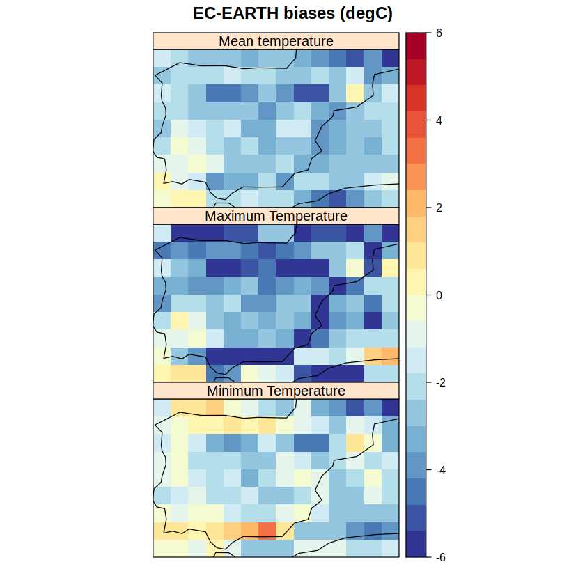
Please note that nearest neighbour interpolation is internally performed within the biasCorrection function (which will be used later) when observations and model grids do not match. Nevertheless, we explicitly do it here for biases calculation. Mean bias of daily mean, maximum and minimum temperature during the historical period are computed with gridArithmetics.
bias.tas <- gridArithmetics(climatology(hist.tas), climatology(y.tas), operator = "-")
bias.tasmax <- gridArithmetics(climatology(hist.tasmax), climatology(y.tasmax), operator = "-")
bias.tasmin <- gridArithmetics(climatology(hist.tasmin), climatology(y.tasmin), operator = "-")
[2023-05-07 16:58:30] - Computing climatology...
[2023-05-07 16:58:30] - Done.
[2023-05-07 16:58:30] - Computing climatology...
[2023-05-07 16:58:30] - Done.
[2023-05-07 16:58:30] - Computing climatology...
[2023-05-07 16:58:30] - Done.
[2023-05-07 16:58:30] - Computing climatology...
[2023-05-07 16:58:30] - Done.
[2023-05-07 16:58:30] - Computing climatology...
[2023-05-07 16:58:30] - Done.
[2023-05-07 16:58:30] - Computing climatology...
[2023-05-07 16:58:30] - Done.
The results are plotted with the spatialPlot function from the visualizeR package.
spatialPlot(suppressMessages(makeMultiGrid(bias.tas, bias.tasmax, bias.tasmin, skip.temporal.check = TRUE)),
            backdrop.theme = "coastline",
            names.attr = c("Mean temperature", "Maximum Temperature", "Minimum Temperature"),
            main = "EC-EARTH biases (degC)", layout = c(1, 3), as.table = TRUE,
            set.min = -6, set.max = 6, at = seq(-6, 6, 12/20), rev.colors = TRUE)
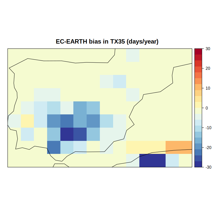
Similarly, we can also visualize the EC-EARTH bias for TX35 (number of days per year with maximum temperature above 35º) during the historical period. This index can be easily computed with the indexGrid function:
# Observed TX35, year by year
index.obs <- redim(indexGrid(tx = y.tasmax, index.code = "TXth", th = 35, time.resolution = "year"),
                   drop = TRUE)
# Simulated TX35, year by year
index.raw <- redim(indexGrid(tx = hist.tasmax, index.code = "TXth", th = 35, time.resolution = "year"),
                   drop = TRUE)

tx35.obs <- climatology(index.obs)  # Mean value
tx35.raw <- climatology(index.raw)  # Mean value
bias.tx35 <- gridArithmetics(tx35.raw, tx35.obs, operator = "-")  # Bias
[2023-05-07 16:58:30] Calculating TXth ...
[2023-05-07 16:58:30] Done
[2023-05-07 16:58:30] Calculating TXth ...
[2023-05-07 16:58:30] Done
[2023-05-07 16:58:30] - Computing climatology...
[2023-05-07 16:58:30] - Done.
[2023-05-07 16:58:30] - Computing climatology...
[2023-05-07 16:58:30] - Done.
spatialPlot(bias.tx35, backdrop.theme = "coastline", main = "EC-EARTH bias in TX35 (days/year)",
            set.min = -30, set.max = 30,
            at = seq(-30, 30, 60/20),
            rev.colors = TRUE)
Bias adjustment#
Three individual adjustments need to be done to get bias-adjusted daily minimum and maximum temperatures with the ISIMIP3 method:
Bias adjustment of mean temperature
Bias adjustment of temperature range
Bias adjustment of temperature skewness
In this example, the three steps are next undertaken to correct both historical and future model simulations.
We start by calculating the temperature range and skewness for the observations and (historical and future) simulations using the gridArithmetics function:
# Range
y.range <- gridArithmetics(y.tasmax, y.tasmin, operator = "-")
x.range <- gridArithmetics(x.tasmax, x.tasmin, operator = "-")
newdata.range <- gridArithmetics(newdata.tasmax, newdata.tasmin, operator = "-")

# Skewness
y.skew <- gridArithmetics(gridArithmetics(y.tas, y.tasmin, operator = "-"), y.range, operator = "/")
x.skew <- gridArithmetics(gridArithmetics(x.tas,x.tasmin, operator = "-"), x.range, operator = "/")
newdata.skew <- gridArithmetics(gridArithmetics(newdata.tas, newdata.tasmin, operator = "-"),
                                newdata.range, operator = "/")
Next, the biasCorrection function is used to perform the three steps mentioned above, by indicating the ISIMIP3 method and related arguments as inputs. Other (methodologically simpler) methods are also available in biasCorrection; the reader is referred to the function documentation for more details.
1.Bias adjustment of daily mean temperature:
# List of arguments that have to be passed to the "biasCorrection" function when using the ISIMIP3 method
isimip3.args = list(lower_bound = NULL,lower_threshold = NULL, upper_bound = NULL,
                    upper_threshold = NULL,  randomization_seed =  NULL,
                    detrend = array(data = TRUE, dim = 1), rotation_matrices = NULL,
                    n_quantiles = 50, distribution = "normal",
                    trend_preservation = array(data = "additive", dim = 1),
                    adjust_p_values = array(data = FALSE, dim = 1), if_all_invalid_use = NULL,
                    invalid_value_warnings = FALSE)

# Adjusting historical simulations
bc.tas.hist <- biasCorrection(y = y.tas, x = x.tas, newdata = x.tas, "precipitation" = FALSE,
                         method = "isimip3", isimip3.args = isimip3.args)
# Adjusting future simulations
bc.tas <- biasCorrection(y = y.tas, x = x.tas, newdata = newdata.tas, "precipitation" = FALSE,
                         method = "isimip3", isimip3.args = isimip3.args)
[2023-05-07 16:58:31] Trying to determine the time zone...
[2023-05-07 16:58:31] Time zone identified and set to GMT
See 'setGridDates.asPOSIXlt' to change the time zone
[2023-05-07 16:58:31] Trying to determine the time zone...
[2023-05-07 16:58:31] Time zone identified and set to GMT
See 'setGridDates.asPOSIXlt' to change the time zone
[2023-05-07 16:58:31] Trying to determine the time zone...
[2023-05-07 16:58:31] Time zone identified and set to GMT
See 'setGridDates.asPOSIXlt' to change the time zone
[2023-05-07 16:58:31] Argument precipitation is set as FALSE, please ensure that this matches your data.
[2023-05-07 16:58:31] Number of windows considered: 1...
[2023-05-07 16:58:31] Bias-correcting 1 members separately...
[2023-05-07 16:58:44] Done.
[2023-05-07 16:58:44] Trying to determine the time zone...
[2023-05-07 16:58:44] Time zone identified and set to GMT
See 'setGridDates.asPOSIXlt' to change the time zone
[2023-05-07 16:58:44] Trying to determine the time zone...
[2023-05-07 16:58:44] Time zone identified and set to GMT
See 'setGridDates.asPOSIXlt' to change the time zone
[2023-05-07 16:58:44] Trying to determine the time zone...
[2023-05-07 16:58:44] Time zone identified and set to GMT
See 'setGridDates.asPOSIXlt' to change the time zone
[2023-05-07 16:58:44] Argument precipitation is set as FALSE, please ensure that this matches your data.
[2023-05-07 16:58:44] Number of windows considered: 1...
[2023-05-07 16:58:44] Bias-correcting 1 members separately...
[2023-05-07 16:58:52] Done.
2.Bias ajustment of the daily temperature range:
# List of arguments that have to be passed to the "biasCorrection" function when using the ISIMIP3 method
isimip3.range.args = list(lower_bound = 0, lower_threshold = 0.01, upper_bound = NULL,
                            upper_threshold = NULL, randomization_seed = NULL,
                            detrend = array(data = FALSE, dim = 1), rotation_matrices =  NULL,
                            n_quantiles = 50, distribution = "rice",
                            trend_preservation = array(data = "mixed", dim = 1),
                            adjust_p_values = array(data = FALSE, dim = 1), if_all_invalid_use = NULL,
                            invalid_value_warnings = FALSE)

# Adjusting historical simulations
bc.range.hist <- biasCorrection(y = y.range, x = x.range, newdata = x.range, "precipitation" = FALSE,
                                method = "isimip3", isimip3.args = isimip3.range.args)
# Adjusting future simulations
bc.range <- biasCorrection(y = y.range, x = x.range, newdata = newdata.range, "precipitation" = FALSE,
                           method = "isimip3", isimip3.args = isimip3.range.args)
[2023-05-07 16:58:52] Trying to determine the time zone...
[2023-05-07 16:58:52] Time zone identified and set to GMT
See 'setGridDates.asPOSIXlt' to change the time zone
[2023-05-07 16:58:52] Trying to determine the time zone...
[2023-05-07 16:58:52] Time zone identified and set to GMT
See 'setGridDates.asPOSIXlt' to change the time zone
[2023-05-07 16:58:52] Trying to determine the time zone...
[2023-05-07 16:58:52] Time zone identified and set to GMT
See 'setGridDates.asPOSIXlt' to change the time zone
[2023-05-07 16:58:53] Argument precipitation is set as FALSE, please ensure that this matches your data.
[2023-05-07 16:58:53] Number of windows considered: 1...
[2023-05-07 16:58:53] Bias-correcting 1 members separately...
[2023-05-07 16:59:00] Done.
[2023-05-07 16:59:00] Trying to determine the time zone...
[2023-05-07 16:59:00] Time zone identified and set to GMT
See 'setGridDates.asPOSIXlt' to change the time zone
[2023-05-07 16:59:00] Trying to determine the time zone...
[2023-05-07 16:59:00] Time zone identified and set to GMT
See 'setGridDates.asPOSIXlt' to change the time zone
[2023-05-07 16:59:00] Trying to determine the time zone...
[2023-05-07 16:59:00] Time zone identified and set to GMT
See 'setGridDates.asPOSIXlt' to change the time zone
[2023-05-07 16:59:00] Argument precipitation is set as FALSE, please ensure that this matches your data.
[2023-05-07 16:59:00] Number of windows considered: 1...
[2023-05-07 16:59:00] Bias-correcting 1 members separately...
[2023-05-07 16:59:08] Done.
3.Bias adjustment of the daily temperature skewness:
# List of arguments that have to be passed to the "biasCorrection" function when using the ISIMIP3 method
isimip3.skew.args  =  list(lower_bound =  c(0), lower_threshold =  c(0.0001), upper_bound =  c(1),
                           upper_threshold =  c(0.9999), randomization_seed =  NULL,
                           detrend =  array(data  =  FALSE, dim = 1), rotation_matrices =  c(NULL),
                           n_quantiles = 50, distribution =  c("beta"),
                           trend_preservation = array(data = "bounded", dim = 1),
                           adjust_p_values = array(data  =  FALSE, dim = 1), if_all_invalid_use  =  c(NULL),
                           invalid_value_warnings  =  FALSE)

# Adjusting historical simulations
bc.skew.hist <- biasCorrection(y = y.skew, x = x.skew, newdata = x.skew, "precipitation" = FALSE,
                          method = "isimip3", isimip3.args = isimip3.skew.args)
# Adjusting future simulations
bc.skew <- biasCorrection(y = y.skew, x = x.skew, newdata = newdata.skew, "precipitation" = FALSE,
                          method = "isimip3", isimip3.args = isimip3.skew.args)
[2023-05-07 16:59:08] Trying to determine the time zone...
[2023-05-07 16:59:08] Time zone identified and set to GMT
See 'setGridDates.asPOSIXlt' to change the time zone
[2023-05-07 16:59:08] Trying to determine the time zone...
[2023-05-07 16:59:08] Time zone identified and set to GMT
See 'setGridDates.asPOSIXlt' to change the time zone
[2023-05-07 16:59:08] Trying to determine the time zone...
[2023-05-07 16:59:08] Time zone identified and set to GMT
See 'setGridDates.asPOSIXlt' to change the time zone
[2023-05-07 16:59:08] Argument precipitation is set as FALSE, please ensure that this matches your data.
[2023-05-07 16:59:08] Number of windows considered: 1...
[2023-05-07 16:59:08] Bias-correcting 1 members separately...
[2023-05-07 16:59:16] Done.
[2023-05-07 16:59:16] Trying to determine the time zone...
[2023-05-07 16:59:16] Time zone identified and set to GMT
See 'setGridDates.asPOSIXlt' to change the time zone
[2023-05-07 16:59:16] Trying to determine the time zone...
[2023-05-07 16:59:16] Time zone identified and set to GMT
See 'setGridDates.asPOSIXlt' to change the time zone
[2023-05-07 16:59:16] Trying to determine the time zone...
[2023-05-07 16:59:16] Time zone identified and set to GMT
See 'setGridDates.asPOSIXlt' to change the time zone
[2023-05-07 16:59:16] Argument precipitation is set as FALSE, please ensure that this matches your data.
[2023-05-07 16:59:16] Number of windows considered: 1...
[2023-05-07 16:59:16] Bias-correcting 1 members separately...
[2023-05-07 16:59:24] Done.
Once these three steps are completed, the bias-adjusted daily maximum and minimum temperature can be obtained as follows:
# Bias-adjusted historical temperatures
bc.tasmin.hist <- gridArithmetics(bc.tas.hist, gridArithmetics(bc.range.hist, bc.skew.hist, operator = "*"),
                                  operator = "-")
bc.tasmax.hist <- gridArithmetics(bc.tasmin.hist, bc.range.hist, operator = "+")

# Bias-adjusted future temperatures
bc.tasmin <- gridArithmetics(bc.tas, gridArithmetics(bc.range, bc.skew, operator = "*"),
                             operator = "-")
bc.tasmax <- gridArithmetics(bc.tasmin, bc.range, operator = "+")
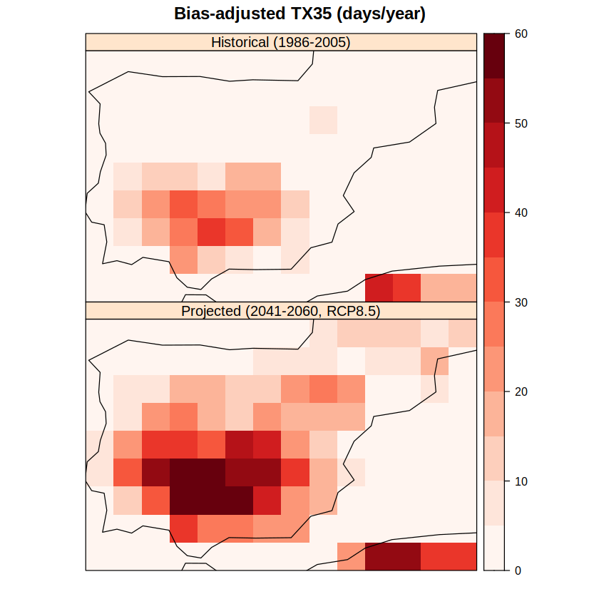
Calculation of extreme temperature indices#
Finally, we use the indexGrid function to compute historical and future TX35 based on the bias-adjusted daily maximum temperature which has been obtained from the application of the ISIMIP3 method.
# Bias-adjusted TX35 for the historical period, year by year
index.hist <- redim(indexGrid(tx = bc.tasmax.hist, index.code = "TXth", th = 35,
                              time.resolution = "year"), drop = TRUE)
tx35.hist <- climatology(index.hist)  # Mean value (number of days/year)

# Bias-adjusted TX35 for the future period of interest, year by year
index.rcp <- redim(indexGrid(tx = bc.tasmax, index.code = "TXth", th = 35,
                             time.resolution = "year"), drop = TRUE)
tx35.rcp <- climatology(index.rcp) # Mean value (number of days/year)
[2023-05-07 16:59:24] Calculating TXth ...
[2023-05-07 16:59:24] Done
[2023-05-07 16:59:24] - Computing climatology...
[2023-05-07 16:59:24] - Done.
[2023-05-07 16:59:24] Calculating TXth ...
[2023-05-07 16:59:24] Done
[2023-05-07 16:59:24] - Computing climatology...
[2023-05-07 16:59:24] - Done.
spatialPlot(makeMultiGrid(tx35.hist, tx35.rcp, skip.temporal.check = TRUE), backdrop.theme = "coastline",
            color.them = "Reds", names.attr = c("Historical (1986-2005)","Projected (2041-2060, RCP8.5)"),
            main = "Bias-adjusted TX35 (days/year)", as.table = TRUE, set.min = 0, set.max = 60, at = seq(0,60,5))
Session info#
sessionInfo()
Show code cell output
R version 3.6.3 (2020-02-29)
Platform: x86_64-conda-linux-gnu (64-bit)
Running under: Fedora Linux 38 (Workstation Edition)

Matrix products: default
BLAS/LAPACK: /home/phanaur/mambaforge/envs/tfg/lib/libopenblasp-r0.3.21.so

locale:
 [1] LC_CTYPE=es_ES.UTF-8          LC_NUMERIC=C
 [3] LC_TIME=es_ES.UTF-8           LC_COLLATE=es_ES.UTF-8
 [5] LC_MONETARY=es_ES.UTF-8       LC_MESSAGES=es_ES.UTF-8
 [7] LC_PAPER=es_ES.UTF-8          LC_NAME=es_ES.UTF-8
 [9] LC_ADDRESS=es_ES.UTF-8        LC_TELEPHONE=es_ES.UTF-8
[11] LC_MEASUREMENT=es_ES.UTF-8    LC_IDENTIFICATION=es_ES.UTF-8

attached base packages:
[1] stats     graphics  grDevices utils     datasets  methods   base

other attached packages:
 [1] rgdal_1.5-16            sp_1.4-5                visualizeR_1.6.1
 [4] climate4R.indices_0.2.0 downscaleR_3.3.3        transformeR_2.1.3
 [7] loadeR_1.7.1            climate4R.UDG_0.2.3     loadeR.java_1.1.1
[10] rJava_1.0-4

loaded via a namespace (and not attached):
 [1] CircStats_0.2-6         bitops_1.0-7            RColorBrewer_1.1-2
 [4] rprojroot_2.0.2         evd_2.3-3               sticky_0.5.6.1
 [7] repr_1.1.3              tools_3.6.3             padr_0.5.3
[10] utf8_1.2.1              R6_2.5.0                sm_2.2-5.6
[13] colorspace_2.0-1        withr_2.4.2             tidyselect_1.1.1
[16] gridExtra_2.3           compiler_3.6.3          glmnet_4.1-1
[19] scales_1.1.1            pbapply_1.4-3           dtw_1.22-3
[22] proxy_0.4-25            rappdirs_0.3.3          pbdZMQ_0.3-5
[25] digest_0.6.27           vioplot_0.3.6           base64enc_0.1-3
[28] jpeg_0.1-8.1            pkgconfig_2.0.3         htmltools_0.5.1.1
[31] akima_0.6-2.1           maps_3.3.0              rlang_0.4.11
[34] shape_1.4.6             mapplots_1.5.1          generics_0.1.0
[37] zoo_1.8-9               jsonlite_1.7.2          dplyr_1.0.6
[40] RCurl_1.98-1.3          magrittr_2.0.1          verification_1.42
[43] dotCall64_1.0-1         Matrix_1.3-3            Rcpp_1.0.6
[46] IRkernel_1.2            munsell_0.5.0           fansi_0.4.2
[49] abind_1.4-5             reticulate_1.27         viridis_0.6.1
[52] lifecycle_1.0.0         MASS_7.3-54             grid_3.6.3
[55] parallel_3.6.3          crayon_1.4.1            udunits2_0.13
[58] lattice_0.20-44         IRdisplay_1.0           convertR_0.2.0
[61] splines_3.6.3           pillar_1.6.1            tcltk_3.6.3
[64] uuid_0.1-4              boot_1.3-28             codetools_0.2-18
[67] glue_1.4.2              evaluate_0.14           latticeExtra_0.6-29
[70] kohonen_3.0.10          data.table_1.14.0       png_0.1-7
[73] vctrs_0.3.8             spam_2.6-0              foreach_1.5.1
[76] gtable_0.3.0            purrr_0.3.4             ggplot2_3.3.3
[79] RcppEigen_0.3.3.9.1     survival_3.2-11         viridisLite_0.4.0
[82] tibble_3.1.2            iterators_1.0.13        SpecsVerification_0.5-3
[85] fields_12.3             deepnet_0.2             ellipsis_0.3.2
[88] easyVerification_0.4.4  here_1.0.1
References#
- Pac
An R package to visualize and communicate uncertainty in seasonal climate prediction - ScienceDirect. https://doi.org/10.1016/j.envsoft.2017.09.008.
- Tes(1,2)
Testing bias adjustment methods for regional climate change applications under observational uncertainty and resolution mismatch - Casanueva - 2020 - Atmospheric Science Letters - Wiley Online Library. https://doi.org/10.1002/asl.978.
- Rba(1,2,3)
The R-based climate4R open framework for reproducible climate data access and post-processing - ScienceDirect. https://doi.org/10.1016/j.envsoft.2018.09.009.
- CRA
CRAN - Package rgdal. https://cran.r-project.org/web/packages/rgdal/index.html.
- GMDa
GMD - Statistical downscaling with the downscaleR package (v3.1.0): contribution to the VALUE intercomparison experiment. https://doi.org/10.5194/gmd-13-1711-2020.
- GMDb
GMD - Trend-preserving bias adjustment and statistical downscaling with ISIMIP3BASD (v1.0). https://doi.org/10.5194/gmd-12-3055-2019.
- UDG(1,2)
UDG-TAP Home. http://meteo.unican.es/udg-tap/home.
- cli22
SantanderMetGroup/climate4R. https://github.com/SantanderMetGroup/climate4R, July 2022.
- CWA+20
Marco Cucchi, Graham P. Weedon, Alessandro Amici, Nicolas Bellouin, Stefan Lange, Hannes Müller Schmied, Hans Hersbach, and Carlo Buontempo. WFDE5: bias-adjusted ERA5 reanalysis data for impact studies. Earth System Science Data, 12(3):2097–2120, September 2020. doi:10.5194/essd-12-2097-2020.