Computing and visualizing regional climate change (temperature vs precipitation) for reference regions

Computing and visualizing regional climate change (temperature vs precipitation) for reference regions#

24/6/2021

M. Iturbide (Santander Meteorology Group. Institute of Physics of Cantabria, CSIC-UC, Santander, Spain).

This notebook reproduces and extends parts of the regional figures of the AR6-WGI Atlas chapter. In particular, the scatter plots of regional climate change temperature vs. precipitation for the AR6 reference regions using CMIP5 and CMIP6 datasets (Figures Atlas.13, 16 ,17, 21, 22, 24, 26 and 29). This notebook builds on other sections of the repository: 1) auxiliary scripts from reproducibility, and 2) CMIP5/6 - CORDEX datasets-aggregated-regionally for the WGI reference regions.

Load packages and functions#

This notebook is based on the R programming language and requires packages:

magrittr to pipe (%>%) sequences of operations
httr to handle URLs and HTTP
lattice and latticeExtra to produce the figures
gridExtra to produce the final panel of plots

library(magrittr)
library(httr)
library(lattice)
library(latticeExtra)
library(gridExtra)

The main function to generate the boxplots and scatterplots is computeFigures, which internally uses functions computeDeltas and computeOffset, all available in this repository. To load these functions in the working environment use the source R base function as follows.

source("../datasets-aggregated-regionally/scripts/computeDeltas.R")
source("../datasets-aggregated-regionally/scripts/computeFigures.R")
source("../datasets-aggregated-regionally/scripts/computeOffset.R")

The scripts are available for download:

Parameter setting#

We define next some parameters, such as the seasons to show in the Precipitation vs Temperature scatterplots. E.g. for boreal winter and summer define:

scatter.seasons <- list(c(12, 1, 2), 6:8)

Select baseline period (e.g. AR6 reference period in this example). Available years in the datasets are 1850-1900 and 1950-2100.

ref.period <- 1995:2014

Select the area, i.e. “land”, “sea” or “landsea”

area <- "land"

Select reference regions (see reference-regions in this repository). Use world to generate global results.

regions <- c("ECA", "EAS"); 

Select a CORDEX domain from the following options: SAM, CAM, NAM, AFR, WAS, EAS, AUS, ANT, ARC, SEA and EUR

cordex.domain <- "EAS"

Finally, select figure axes ranges (ylim for temperature, xlim for precipitation percentage). Leave it as NULL for automatic axes ranges

ylim <- NULL
xlim <- NULL

Compute delta changes and figures#

We are ready to apply the computeFigures function.

fig <- computeFigures(regions = regions,
                      cordex.domain = cordex.domain,
                      area = area, 
                      ref.period = ref.period, 
                      scatter.seasons = scatter.seasons,
                      xlim = xlim,
                      ylim = ylim)

The output of the above call (fig) is a list of trellis class objects that can be easily arranged and displayed using the grid.arrange function from the gridExtra library.

do.call("grid.arrange", fig)

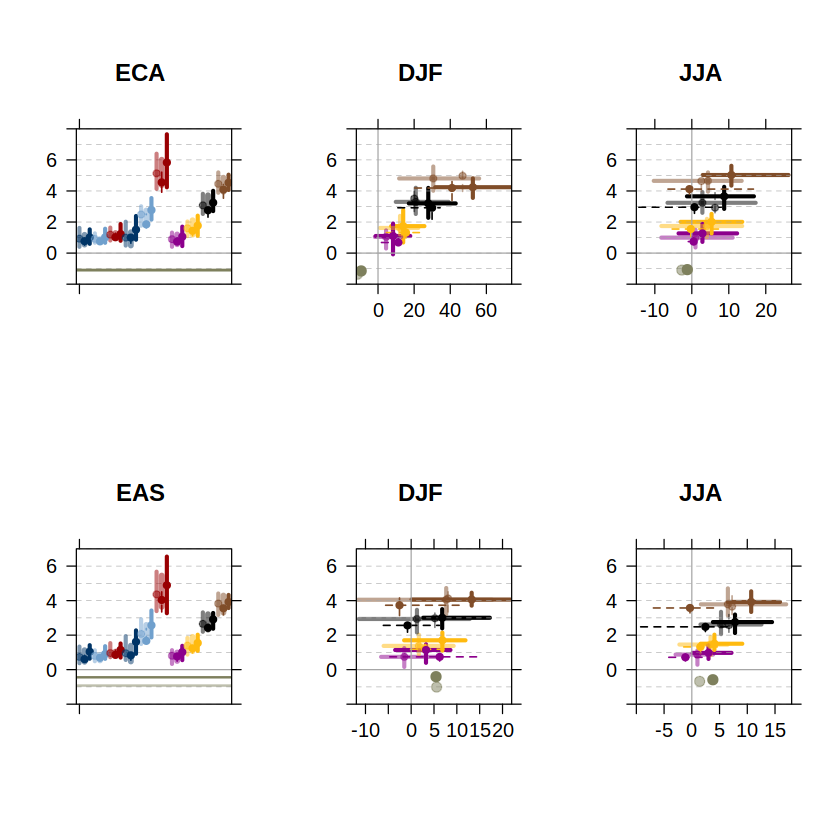
../_images/6123a56ef8d1a1b71916df3ed686f4090b322e7d6c182ed622002d551748bdc3.png

The legend and axis label information of these panels is the one shown in the AR6-WGI Atlas chapter figures. The first column shows the annual temperature delta changes. The second and third columns, the scatterplots of the seasonal temperature and precipitation changes. Each row corresponds to a different reference region (ECA and EAS in this worked example).

We can now export the Figure as PDF. There are other export options such as png (type ?pdf for help). The Cairo package provides other export options.

outfilename <- sprintf("%s_%s_baseperiod_%s_ATvsAP.pdf",
  cordex.domain, area, paste(range(ref.period), collapse = "-")
)

pdf(outfilename, width = (length(scatter.seasons)+1)*10/2*0.85, height = length(regions)*10/2*0.85)
  do.call("grid.arrange", fig)
dev.off()

png: 2

Play with arguments width and height to create different PDF sizes.

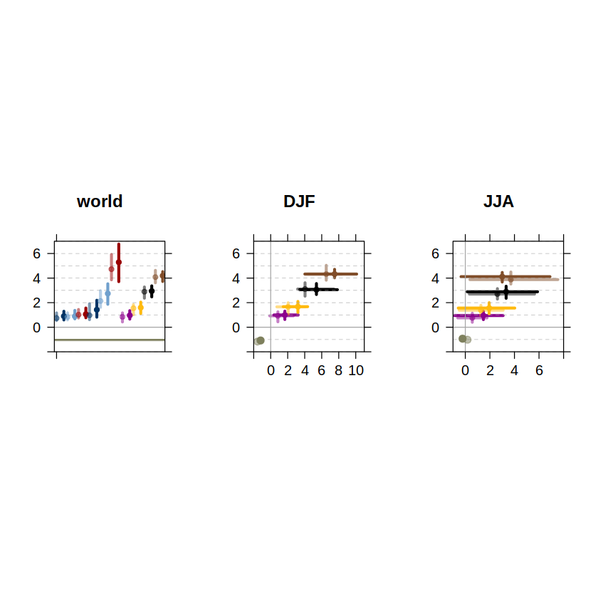
Set the object cordex.domain as FALSE to exclude CORDEX from the final figure. For example, in order to compute global delta changes, we can set:

regions <- c("world")
cordex.domain <- FALSE

fig.w <- computeFigures(regions = regions,
                      cordex.domain = cordex.domain,
                      area = area, 
                      ref.period = ref.period, 
                      scatter.seasons = scatter.seasons,
                      xlim = xlim,
                      ylim = ylim)

do.call("grid.arrange", fig.w)

../_images/9bdeb65167cdf0d573f96123438e6e304441356e03e52223857ed4f6fc7af10d.png

We have easily reproduced parts of the AR6-WGI Atlas chapter figures using the function computeFigures. To extend the results shown in the Atlas chapter, just use different parameter settings above, e.g. additional seasons, alternative baselines, etc.

Furthermore, functions computeDeltas and computeOffset (which are internally applied by computeFigures) can also be applied directly to obtain the data behind the boxplots/scatterplots allowing for further plotting options, which we explore next.

Data matrices of delta changes#

In this last example, we will compute CMIP5 annual temperature changes for different Global Warming Levels. Therefore, the following parameters are set.

project <- "CMIP5" # other options are CMIP6 and CORDEX
experiment <- "rcp85" 
var <- "tas"
season <- 1:12
ref.period <- 1986:2005
periods <- c("1.5", "2", "3", "4") 
area <- "land"
region <- c("NSA", "SES")
cordex.domain <- "SAM"

WL.cmip5 <- computeDeltas(project = project, 
                          var = var, 
                          experiment = experiment, 
                          season = season, 
                          ref.period = ref.period, 
                          periods = periods, 
                          area = area, 
                          region = region, 
                          cordex.domain = cordex.domain)

The cordex.domain parameter will be ignored unless the project is CORDEX (project <- "CORDEX").

The output of the computeDeltas function is a list of matrices, each corresponding to a different reference region. Each column of the matrix corresponds to the warming levels set before. E.g. for the SES region:

WL.cmip5$SES

Show code cell output Hide code cell output

A matrix: 28 × 4 of type dbl
	rcp85	rcp85	rcp85	rcp85
ACCESS1-0_r1i1p1	0.9483292	1.4299875	2.460746	3.316342
ACCESS1-3_r1i1p1	1.1470417	1.5117708	2.427108	3.273229
bcc-csm1-1_r1i1p1	0.3947792	1.0546292	1.967492	3.097608
bcc-csm1-1-m_r1i1p1	0.7028111	0.8685500	1.773425	2.922742
CanESM2_r1i1p1	1.0021815	1.4546208	2.752146	3.829083
CCSM4_r1i1p1	0.6210013	1.1669375	2.127387	3.339333
CESM1-BGC_r1i1p1	0.6845792	1.1676000	2.062329	3.313937
CMCC-CM_r1i1p1	0.7409458	1.3561125	2.278021	3.326538
CMCC-CMS_r1i1p1	0.9705500	1.4402042	2.370708	3.405425
CNRM-CM5_r1i1p1	0.8366167	1.3981083	2.189842	3.274875
CSIRO-Mk3-6-0_r1i1p1	1.0670042	1.5795292	2.844288	3.816117
EC-EARTH_r12i1p1	0.5381833	0.8834292	1.876096	2.958067
GFDL-CM3_r1i1p1	0.9836042	1.6451250	2.691879	3.626942
GFDL-ESM2G_r1i1p1	1.2233958	1.7253083	2.800908	NA
GFDL-ESM2M_r1i1p1	1.0523500	1.6082625	2.808379	NA
HadGEM2-CC_r1i1p1	1.0337867	1.4512784	2.591049	3.326278
HadGEM2-ES_r1i1p1	0.8743534	1.2426534	2.104303	3.121641
inmcm4_r1i1p1	1.2622667	1.8953958	2.734242	NA
IPSL-CM5A-LR_r1i1p1	0.6381226	1.0454042	2.164887	3.292792
IPSL-CM5A-MR_r1i1p1	0.6028292	1.2632875	2.462396	3.771575
IPSL-CM5B-LR_r1i1p1	0.6907500	1.1536042	1.970087	2.876000
MIROC-ESM_r1i1p1	0.8756792	1.4630167	2.241883	3.352113
MIROC-ESM-CHEM_r1i1p1	0.9714833	1.4255125	2.399029	3.431421
MIROC5_r1i1p1	1.0668667	1.3530708	2.071171	NA
MPI-ESM-LR_r1i1p1	0.6644583	1.1644125	2.401737	3.817287
MPI-ESM-MR_r1i1p1	0.7945167	1.3526292	2.587158	3.999304
MRI-CGCM3_r1i1p1	0.8660792	1.4304833	2.233550	NA
NorESM1-M_r1i1p1	0.9928250	1.5723208	2.492021	NA

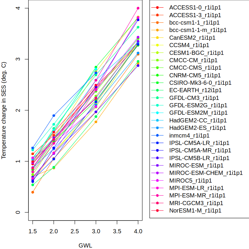
Let’s plot the results for this region and each CMIP5 model.

par(mar=c(4, 4, 0, 15), xpd=TRUE) # make room for the legend
plot(NA, xlim=c(1.5, 4), ylim=c(0,4), xlab = "GWL", ylab = "Temperature change in SES (deg. C)", type = "n")
model.names <- row.names(WL.cmip5$SES)
n.models <- length(model.names)
line.colors <- rainbow(n.models)
gwls <- as.numeric(periods)
for (i in 1:n.models){
    lines(gwls, WL.cmip5$SES[i,], col = line.colors[i])
    points(gwls, WL.cmip5$SES[i,], col = line.colors[i], pch=16)
}
legend("topright", legend=model.names, pch=16, lty=1, col=line.colors, inset=c(-1,0))

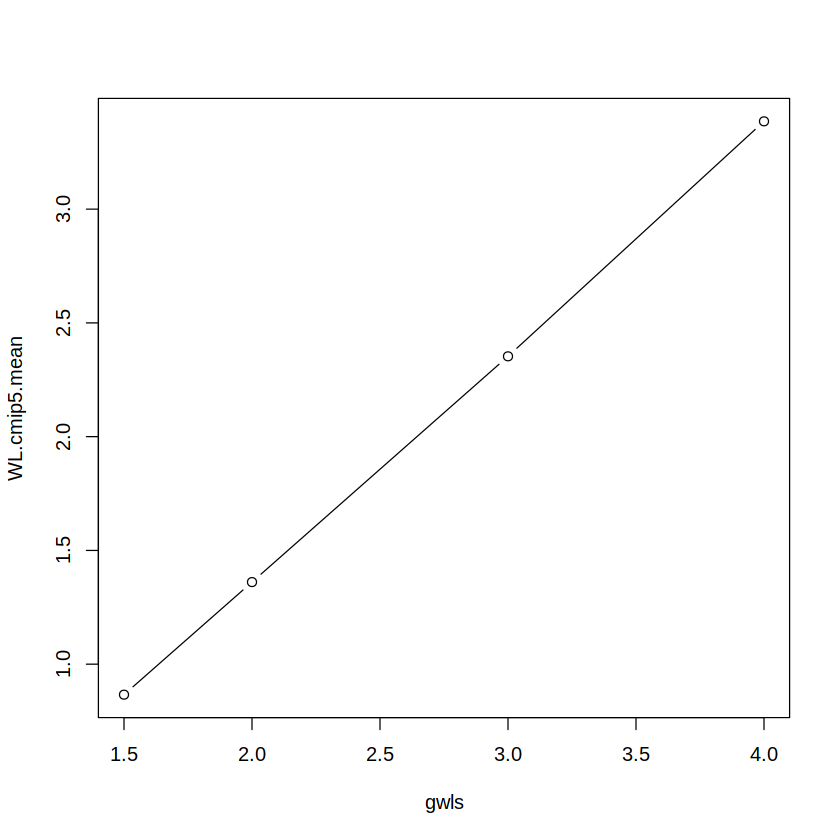
../_images/f1624904bb9079b23e2230b1cc8301e931eec0fc6abe9dcec6cedbd191df0c1c.png

Once the data is obtained, the user is free to apply any additional operations. For instance, in the next cell we will compute the ensemble mean for the SES region using the apply function.

WL.cmip5.mean <- apply(WL.cmip5$SES, 2, mean, na.rm = T)
plot(gwls, WL.cmip5.mean, type = "b")

../_images/1545cda5506caf1048a862dc387a338275f6e30a47a6a3d21e7abe1a96ff40aa.png

Use a for or a lapply loop to apply the same operation for all available regions:

WL.cmip5.mean <- lapply(WL.cmip5, function(x) apply(x, 2, mean, na.rm = T))

Convert from list to data.frame and add WL names:

df <- data.frame("WL" = gwls, WL.cmip5.mean)
df

A data.frame: 4 × 3
WL	NSA	SES
<dbl>	<dbl>	<dbl>
1.5	1.080562	0.8659782
2.0	1.673109	1.3608302
3.0	2.962334	2.3530096
4.0	4.307700	3.3858477

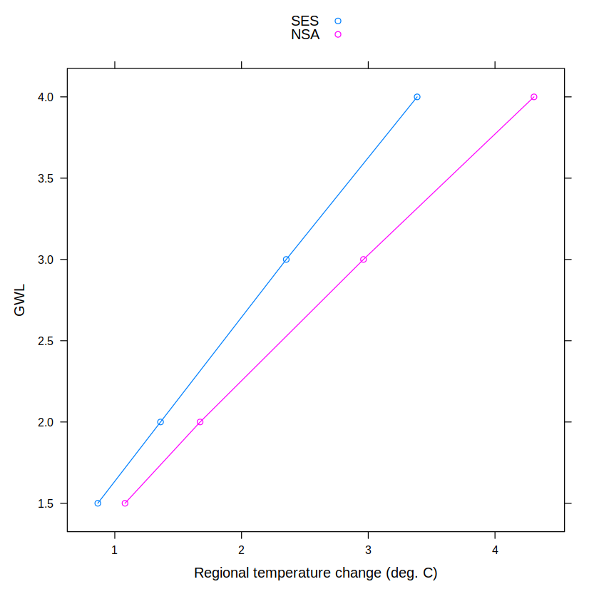
We can use this data frame to illustrate the lattice plotting functionalities.

xyplot(WL~SES + NSA, data = df, 
       xlab = "Regional temperature change (deg. C)", ylab = "GWL",
       type = "b",
       auto.key = TRUE)

../_images/1eccff3dcc70060ff5f2426f25b3a80823632344a1e1177cec127f7ab0555699.png