Using the Atlas reference grids in R

# Atlas notebooks

***

> This notebook reproduces and extends parts of the figures and products of the AR6-WGI Atlas. It is part of a notebook collection available at https://github.com/IPCC-WG1/Atlas for reproducibility and reusability purposes. This work is licensed under a [Creative Commons Attribution 4.0 International License](http://creativecommons.org/licenses/by/4.0).
>
> ![Creative Commons License >](https://i.creativecommons.org/l/by/4.0/88x31.png)

Using the Atlas reference grids in `R`#

22/07/2021

M. Iturbide (Santander Meteorology Group, Instituto de Física de Cantabria, CSIC-UC, Santander, Spain)

This is a simple example which illustrates how the Atlas reference grids can be used in R for both interpolation and land/sea separation of the simulations provided by a global climate model.

Load libraries#

The following climate4R (C4R hereafter) libraries are needed to run this notebook:

loadeR [An R Package to Visualize and Communicate Uncertainty in Seasonal Climate Prediction - ScienceDirect] to load data
visualizeR to display the results
convertR to change units

library(loadeR)
library(visualizeR)
library(convertR)

Load the reference land/sea mask#

The global reference 1º land/sea mask used for the generation of part of the Atlas products can be loaded directly from this repository with the loadGridData function:

# global reference 1º land/sea mask
mask <- loadGridData("../reference-grids/land_sea_mask_1degree.nc4", var = "sftlf")

[2023-05-07 17:03:11] Defining geo-location parameters

[2023-05-07 17:03:11] Defining time selection parameters

NOTE: Undefined Dataset Time Axis (static variable)

[2023-05-07 17:03:11] Retrieving data subset ...

[2023-05-07 17:03:11] Done

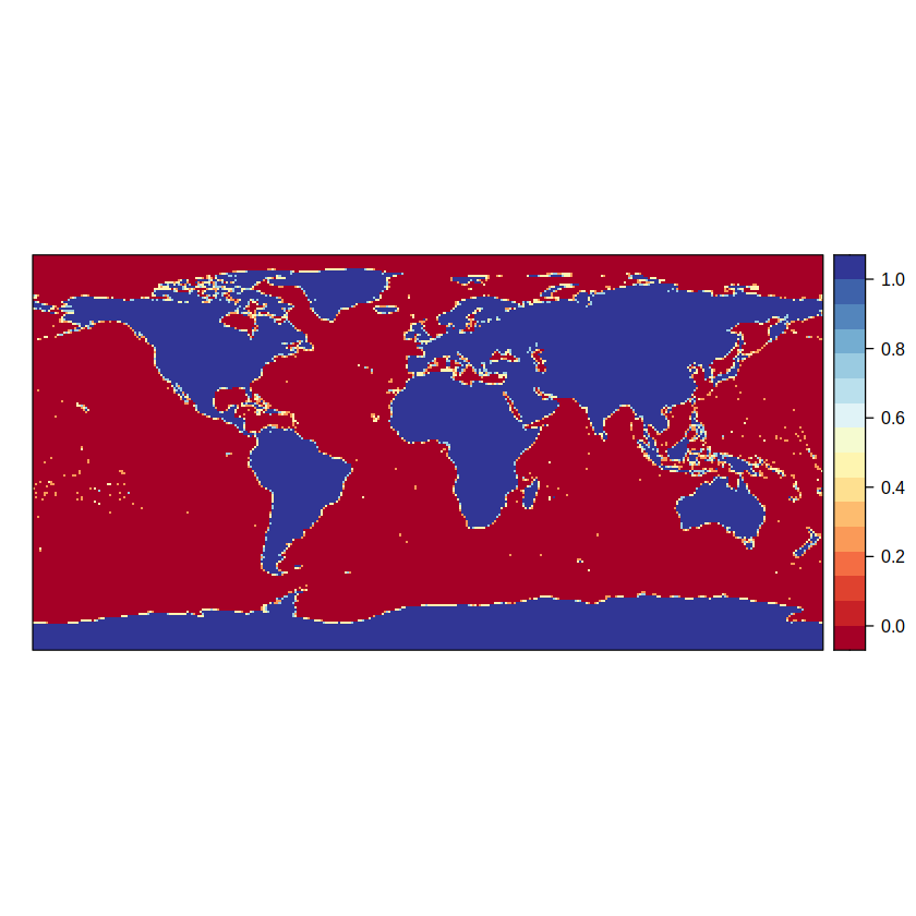
This mask is a C4R grid object which contains the land fraction (a value in between 0 and 1) in each gridbox.

# plotting mask
spatialPlot(mask)

../_images/e48e5a6f09735dc879bb581085c4cf9b86d6fc60a5ee6b6214e2fad97a5d4b91.png

Load model data#

For this example we will use the global mean temperature from the CanESM5 model, which is provided at a monthly time resolution in a netCDF file in the auxiliary-material folder. In particular, we focus on the 2000-2010 period, which can be specified with the years argument in the loadGridData function:

# loading global mean temperature
tas <- loadGridData("auxiliary-material/CMIP6Amon_tas_CanESM5_r1i1p1f1_historical_gn_185001-201412.nc", 
                    var = "tas", years = 2000:2010) 

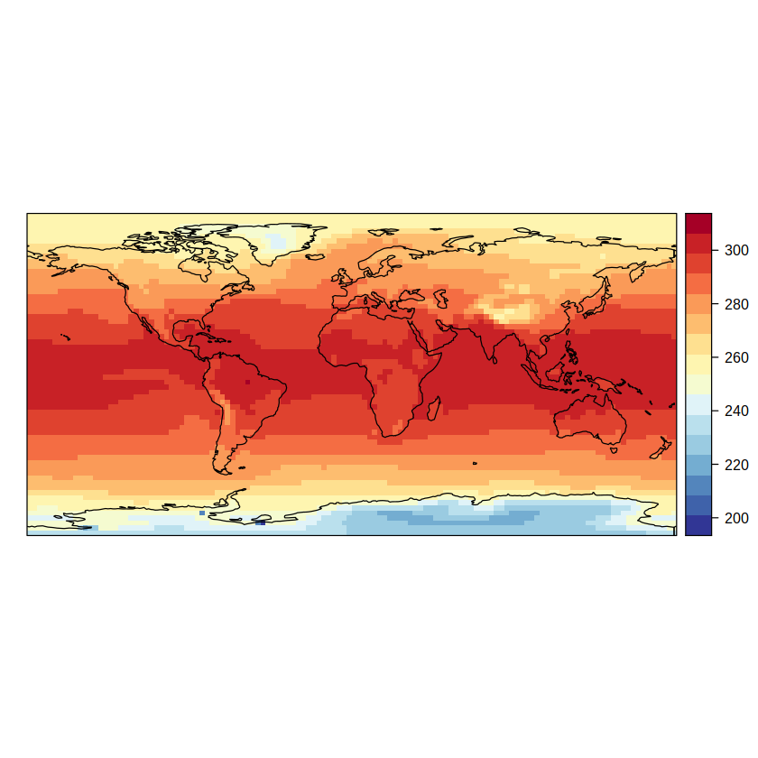
Let’s plot the climatology for the analyzed period:

# plotting climatology
spatialPlot(climatology(tas), backdrop.theme = "coastline", rev.colors = TRUE)

Interpolation#

The global mean temperature we have just loaded comes in the original grid of the CanESM5 model, which has a spatial resolution of about 2.8º:

attributes(getGrid(tas))$resX
attributes(getGrid(tas))$resY

2.8125

2.78932694727723

In order to apply the reference 1º land/sea mask to these data and retain only land temperatures, we need first to interpolate the CanESM5 model to the grid of the mask, which can be done with the interpGrid function. We will use in this example bilinear interpolation; however, other interpolation methods are also available in interpGrid.

# Note: This cell may take a while to run 
tas.i <- interpGrid(tas, getGrid(mask), method = "bilinear")

Warning message in interpGrid(tas, getGrid(mask), method = "bilinear"):
“The new longitudes are outside the data extent”

Warning message in interpGrid(tas, getGrid(mask), method = "bilinear"):
“The new latitudes are outside the data extent”

[2023-05-07 17:03:17] Performing bilinear interpolation... may take a while

[2023-05-07 17:03:22] Done

attributes(getGrid(tas.i))$resX
attributes(getGrid(tas.i))$resY

1

Apply the mask to the data#

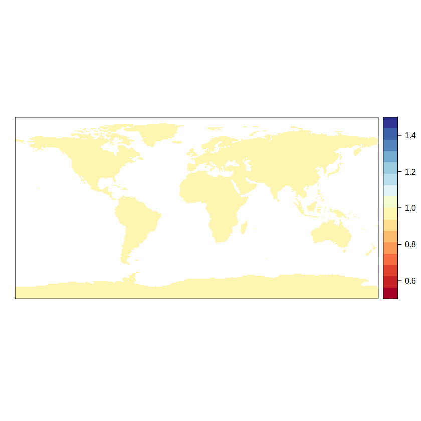
The binaryGrid function assigns two user-provided values (here NA and 1) to a given C4R grid object according to a threshold and condition. We use it here to obtain a new binary land/sea mask with 1 over land and NA over sea. Note that a threshold of 0.999 (99.9%) land fraction is used to define land/sea grid points.

# binary 1º land/sea mask
land <- binaryGrid(mask, condition = "GT", threshold = 0.999, values = c(NA, 1))
spatialPlot(land)

../_images/154145593e09a72c959d11c6d67bc7254917f43cd2ae304cc35ca3cf439acb58.png

In order to apply this binary mask to our temperature data, we need that both C4R grid objects have the same dimensions. Therefore, we resize the binary mask to match the time dimension of tas.i:

masktimes <- rep(list(land), getShape(tas.i, "time"))
mask2apply <- bindGrid(masktimes, dimension = "time")

Warning message in value[[3L]](cond):
“time dimension could not be sorted!”

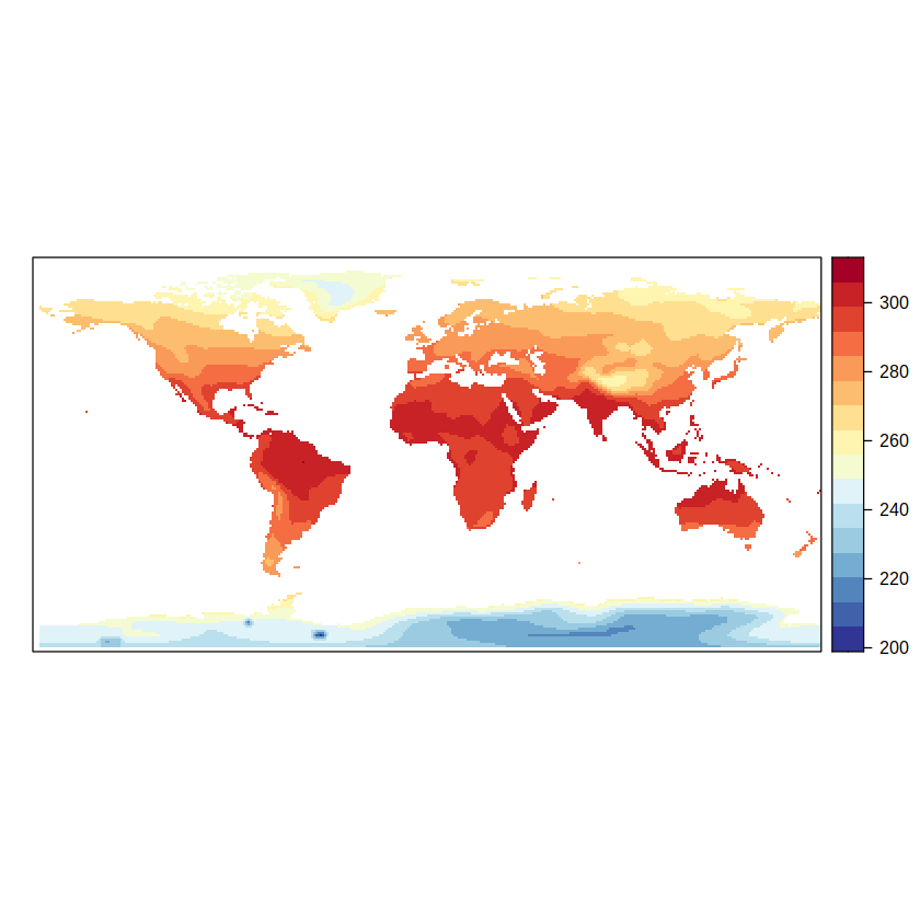
At this point, we can already use the gridArithmetics function to multiply the binary land/sea mask and the temperature data, making NA over sea in the latter.

tas.i.land <- gridArithmetics(tas.i, mask2apply, operator = "*")

# final land-only temperature data
spatialPlot(climatology(tas.i.land), rev.colors = TRUE)  

[2023-05-07 17:03:25] - Computing climatology...

[2023-05-07 17:03:25] - Done.

../_images/abe95d74a2bfebaf6a6c26f50a0cde6f78701593636068c67c10cbc1194b87c8.png

Masked vs. non masked time-series#

Next we compare the monthly time-series of mean temperature, spatially averaged over the entire globe (non masked: tas.i) and only over land regions (masked: tas.i.land):

# monthly time-series (in K)
temporalPlot(tas.i, tas.i.land, x.axis = "index")

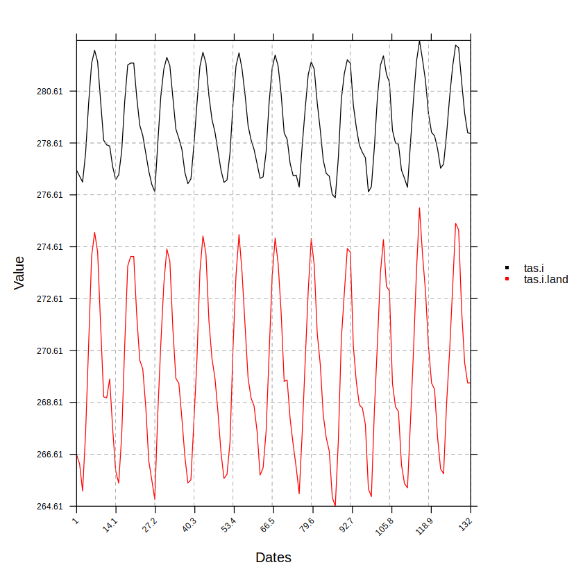
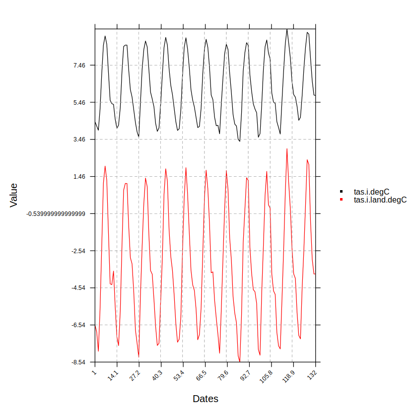
../_images/4197d09c3b73acf9f38b8cccb611d192f8b3aed56008607f9dd66b423e2f44c6.png

Note that temperature is in K units. The udConvertGrid function from the convertR package allows for easily passing from K to Celsius degrees:

# monthly time-series (in Celsius degrees)
tas.i.degC <- udConvertGrid(tas.i, new.units = "degC")
tas.i.land.degC <- udConvertGrid(tas.i.land, new.units = "degC")
temporalPlot(tas.i.degC, tas.i.land.degC, x.axis = "index")

../_images/946551b25033cb79e605894bb3207a6a94454aafc586baaf712fdebbea222d04.png

Session info#

sessionInfo()

Show code cell output Hide code cell output

R version 3.6.3 (2020-02-29)
Platform: x86_64-conda-linux-gnu (64-bit)
Running under: Fedora Linux 38 (Workstation Edition)

Matrix products: default
BLAS/LAPACK: /home/phanaur/mambaforge/envs/tfg/lib/libopenblasp-r0.3.21.so

locale:
 [1] LC_CTYPE=es_ES.UTF-8          LC_NUMERIC=C                 
 [3] LC_TIME=es_ES.UTF-8           LC_COLLATE=es_ES.UTF-8       
 [5] LC_MONETARY=es_ES.UTF-8       LC_MESSAGES=es_ES.UTF-8      
 [7] LC_PAPER=es_ES.UTF-8          LC_NAME=es_ES.UTF-8          
 [9] LC_ADDRESS=es_ES.UTF-8        LC_TELEPHONE=es_ES.UTF-8     
[11] LC_MEASUREMENT=es_ES.UTF-8    LC_IDENTIFICATION=es_ES.UTF-8

attached base packages:
[1] stats     graphics  grDevices utils     datasets  methods   base     

other attached packages:
[1] convertR_0.2.0      udunits2_0.13       visualizeR_1.6.1   
[4] transformeR_2.1.3   loadeR_1.7.1        climate4R.UDG_0.2.3
[7] loadeR.java_1.1.1   rJava_1.0-4        

loaded via a namespace (and not attached):
 [1] viridis_0.6.1           maps_3.3.0              jsonlite_1.7.2         
 [4] viridisLite_0.4.0       SpecsVerification_0.5-3 dotCall64_1.0-1        
 [7] kohonen_3.0.10          sm_2.2-5.6              sp_1.4-5               
[10] latticeExtra_0.6-29     pillar_1.6.1            lattice_0.20-44        
[13] glue_1.4.2              RcppEigen_0.3.3.9.1     uuid_0.1-4             
[16] digest_0.6.27           RColorBrewer_1.1-2      colorspace_2.0-1       
[19] htmltools_0.5.1.1       Matrix_1.3-3            pkgconfig_2.0.3        
[22] padr_0.5.3              purrr_0.3.4             scales_1.1.1           
[25] jpeg_0.1-8.1            CircStats_0.2-6         dtw_1.22-3             
[28] tibble_3.1.2            proxy_0.4-25            generics_0.1.0         
[31] ggplot2_3.3.3           ellipsis_0.3.2          repr_1.1.3             
[34] verification_1.42       pbapply_1.4-3           magrittr_2.0.1         
[37] crayon_1.4.1            easyVerification_0.4.4  evaluate_0.14          
[40] fansi_0.4.2             MASS_7.3-54             tools_3.6.3            
[43] data.table_1.14.0       lifecycle_1.0.0         munsell_0.5.0          
[46] akima_0.6-2.1           compiler_3.6.3          mapplots_1.5.1         
[49] rlang_0.4.11            grid_3.6.3              RCurl_1.98-1.3         
[52] pbdZMQ_0.3-5            IRkernel_1.2            spam_2.6-0             
[55] bitops_1.0-7            tcltk_3.6.3             base64enc_0.1-3        
[58] boot_1.3-28             vioplot_0.3.6           gtable_0.3.0           
[61] abind_1.4-5             R6_2.5.0                gridExtra_2.3          
[64] zoo_1.8-9               dplyr_1.0.6             utf8_1.2.1             
[67] parallel_3.6.3          IRdisplay_1.0           Rcpp_1.0.6             
[70] fields_12.3             vctrs_0.3.8             png_0.1-7              
[73] tidyselect_1.1.1       

References#

Pac: An R package to visualize and communicate uncertainty in seasonal climate prediction - ScienceDirect. https://doi.org/10.1016/j.envsoft.2017.09.008.