Computing and visualization of precipitation linear trends during the observed period (1980-2014)

# Atlas notebooks

***

> This notebook reproduces and extends parts of the figures and products of the AR6-WGI Atlas. It is part of a notebook collection available at https://github.com/IPCC-WG1/Atlas for reproducibility and reusability purposes. This work is licensed under a [Creative Commons Attribution 4.0 International License](http://creativecommons.org/licenses/by/4.0).
>
> ![Creative Commons License >](https://i.creativecommons.org/l/by/4.0/88x31.png)

Computing and visualization of precipitation linear trends during the observed period (1980-2014)#

07/07/2021

J. Baño-Medina (Santander Meteorology Group, Instituto de Física de Cantabria, CSIC-UC, Santander, Spain)

We present an illustrative example to use the climate4R framework to depict the observed linear trends and the time series of precipitation anomalies over a selected time period for the W5E5 observational dataset. North America is used as an example target region. Indications are also provided to apply the methodology to other variables, such as temperature.

Load packages#

This notebook relies on several climate4R packages. We start by extending the Java memory allocation, which will be used by loadeR

options(java.parameters = "-Xmx8g")
library(loadeR)
library(transformeR)
library(visualizeR) # spatialPlot
library(geoprocessoR)
library(climate4R.indices) # linearTrend

Along with other libraries, namely:

magrittr is used to pipe (%>%) sequences of data operations
gridExtra provides plotting functionalities
sp and rgdal provide geospatial tools
RColorBrewer provides color palettes

library(magrittr)
library(sp)
library(RColorBrewer)
library(rgdal) # readOGR

Load static data#

We will load the polygons of the IPCC [Atlas/Reference-Regions at Main · IPCC-WG1/Atlas]:

regs <- get(load("../reference-regions/IPCC-WGI-reference-regions-v4_R.rda")) %>% as("SpatialPolygons")

In this notebook we will focus on a set of regions in North America. We will use the following character vector of the target region names to select them. Change it accordingly to adapt this notebook for other regions.

regs.area <- c("NWN", "NEN", "WNA", "CNA","ENA","NCA") # North America regions

We can now extract the subset of regions and show their outline as follows:

regs <- regs[regs.area]
plot(regs)

../_images/f0600e7bf7187af204d186c695aa3b59712e41774b2ba164b86f3a513f01d0c6.png

We load also the coastlines, to be used in the spatial maps below. These are available in the auxiliary-material folder:

coast <- readOGR("auxiliary-material/WORLD_coastline.shp") 

OGR data source with driver: ESRI Shapefile 
Source: "/home/phanaur/github/Atlas/notebooks/auxiliary-material/WORLD_coastline.shp", layer: "WORLD_coastline"
with 127 features
It has 2 fields

Load observations from the User Data Gateway#

This section takes long to execute due to intensive remote data loading. See the next section (Load data from file) to load these data from a local copy available in the repository and continue with the notebook operations.

The Santander Climate Data Service (SCDS) [Inicio | Servicio Climático de Datos] archives and provides access to a variety of climate datasets and contributes to international infrastructures, serving e.g. as data node for the Earth System Grid Federation (ESGF) or the IPCC Data Distribution Center (IPCC-DDC). This service is maintained by the Santander Meteorology Group (University of Cantabria - CSIC) and includes a THREDDS Data Server for remote data access with seamless integration with the climate4R framework for climate data postprocessing. This integration, the User Data Gateway (UDG), is handled by the climate4R.UDG [climate4R.UDG, 2022] package, loaded automatically by the loadeR [What Is loadeR?, 2022] package, which provides user-friendly access to a variety of remote data sources.

To load data stored in the User Data Gateway (similar to loading data from a local directory), we first list the available datasets with function UDG.datasets:

UDG.datasets()$OBSERVATIONS

Label names are returned, set argument full.info = TRUE to get more information

'WATCH_WFDEI'
'PIK_Obs-EWEMBI'
'E-OBS_v14_0.50regular'
'E-OBS_v14_0.44rotated'
'E-OBS_v14_0.25regular'
'E-OBS_v14_0.22rotated'
'E-OBS_v17_0.50regular'
'E-OBS_v17_0.44rotated'
'E-OBS_v17_0.25regular'
'E-OBS_v17_0.22rotated'
'E-OBS_v21e_0.10regular'
'UC-Spain02_11'
'UC-Spain02_22'
'UC-Spain02_44'
'GPCCmon'
'GPCC'
'GPCPmon'
'GPCP'
'CRU-TS'
'BEST'
'BESTmon'
'W5E5'

We see that, among others, the W5E5 dataset [WFDE5 over Land Merged with ERA5 over the Ocean (W5E5)] is available from the UDG. This dataset is global, but we can load just the region of interest. In this case, we provide the limits for a North American lon-lat window:

lonLim <- c(168.0, -50)
latLim <- c(2.2, 85)

We will also set the analysis period to 1980-2014:

years <- 1980:2014

You can check the available variables in a dataset and other basic information using the dataInventory function.

dataInventory("W5E5")

The standard names used in climate4R (passed to function loadGridData) can be consulted as follows:

C4R.vocavulary()

The variable of interest in this notebook is precipitation:

var <- "pr"

To load W5E5 we would just input the corresponding label to the dataset argument in loadGridData. In order to save memory, we load the data year by year in a loop and perform annual aggregation in each iteration. After using bindGrid (to join the yearly data sets) we end up with a climate4R Grid object containing yearly averages for the region selected. The following piece of code takes about 1 minute per year loaded (depends on your network connection speed).

grid.list <- list()
for (year in years){
    message(" ** Reading year ", year)
    grid.list[[as.character(year)]] <- loadGridData(
        dataset = "W5E5", var = var,
        latLim = latLim, lonLim = lonLim, years = year
    ) %>%
    aggregateGrid(aggr.y = list(FUN = "mean", na.rm = TRUE)) 
}
grid <- bindGrid(grid.list, dimension = "time")                                         

This operation takes a long time, therefore it is convenient to save the resulting data. We can export the final dataset to NetCDF using the loadeR.2nc library, which provides the function grid2nc.

library(loadeR.2nc)
grid2nc(grid, NetCDFOutFile = "auxiliary-material/W5E5_NorthAmerica_pr_1980-2014_yearly.nc4")

The resulting NetCDF is available as auxiliary material in this repository, therefore the previous data loading step can be skipped.

Load data from file#

Skip this section if you sucessfully loaded your data from the User Data Gateway. For a fast loading of the required data, you can use a copy of the yearly averaged precipitation available in the auxiliary-material folder:

grid <- loadGridData("auxiliary-material/W5E5_NorthAmerica_pr_1980-2014_yearly.nc4", var = "pr")

### Plot climatology

We can start by plotting the climatology of precipitation for the selected period and region. We define the geographical projection (WGS84) the same as the reference regions.

grid <- setGridProj(grid = grid, proj = proj4string(regs))

Warning message in proj4string(regs):
“CRS object has comment, which is lost in output”

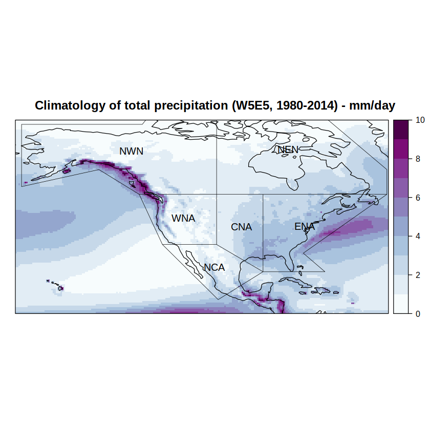
We compute the climatology by calling the climatology function and then use spatialPlot from library visualizeR to depict it. Note that we introduce the IPCC regions of interest in the sp.layout argument.

spatialPlot(climatology(grid),
            at = seq(0, 10, 1), 
            set.min = 0,
            set.max = 10,
            backdrop.theme = "coastline",
            col.regions = brewer.pal(n = 9, "BuPu") %>% colorRampPalette(),
            main = paste0("Climatology of total precipitation (W5E5, ", min(years), "-", max(years), ") - mm/day"),
            sp.layout = list(
                list(regs, first = FALSE, lwd = 0.6),
                list("sp.text", coordinates(regs), names(regs), first = FALSE, cex = 1)
))

[2023-05-07 16:59:34] - Computing climatology...

[2023-05-07 16:59:34] - Done.

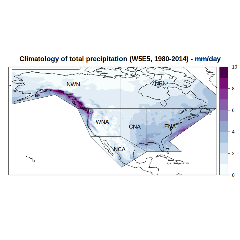
../_images/e499ba2464cb322977e179cbbd3fe0724a9c18455c700a1e99458e8524bb5ebd.png

We can use the overGrid function to mask the values outside the IPCC regions of interest to this use-case.

grid %<>% overGrid(regs)

Warning message in showSRID(uprojargs, format = "PROJ", multiline = "NO"):
“Discarded datum Unknown based on WGS84 ellipsoid in CRS definition”

Compare the resulting plot (same code as above):

spatialPlot(climatology(grid),
            at = seq(0, 10, 1), 
            set.min = 0,
            set.max = 10,
            backdrop.theme = "coastline",
            col.regions = brewer.pal(n = 9, "BuPu") %>% colorRampPalette(),
            main = paste0("Climatology of total precipitation (W5E5, ", min(years), "-", max(years), ") - mm/day"),
            sp.layout = list(
                list(regs, first = FALSE, lwd = 0.6),
                list("sp.text", coordinates(regs), names(regs), first = FALSE, cex = 1)
))

[2023-05-07 16:59:35] - Computing climatology...

[2023-05-07 16:59:35] - Done.

../_images/ac2b470a128d652a9cc6653add5f861a57d9e204c91e1ba5ab53a433779e8639.png

Compute and plot trends#

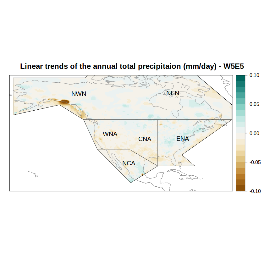
Now, trends can be computed by means of the linearTrend function, which fits a linear model at gridbox level and returns all the involved statistics, including the p-value of the estimated slope. We subset the slope (“b”) among all the statistics returned, by calling subsetGrid.

trendGrid <- linearTrend(grid) %>% subsetGrid(var = "b")

The slope of the linear trend is estimated based on the temporal resolution of the data. Please consider using the function aggregateGrid prior to the call of linearTrend to adequate the data to your resolution of interest.

[2023-05-07 16:59:35] - Computing climatology...

[2023-05-07 16:59:35] - Done.

Warning message:
“Only one grid passed as input. Nothing was done”

We could save these climate products as NetCDF files using the loadeR.2nc library.

grid2nc(trendGrid, NetCDFOutFile = "trends.nc4")

We rely again on spatialPlot from visualizeR, to show the map of trends.

spatialPlot(trendGrid, 
            col.regions = brewer.pal(n = 9, "BrBG") %>% colorRampPalette(),
            at = seq(-0.1, 0.1, 0.01), 
            set.min = -0.1,
            set.max = 0.1,
            main = paste("Linear trends of the annual total precipitaion (mm/day) - W5E5"),
            sp.layout = list(  
            list(regs, first = FALSE, lwd = 0.6),
            list(coast, col = "gray50", first = FALSE, lwd = 0.6),  
            list("sp.text", coordinates(regs), names(regs), first = FALSE, cex = 1)
))

../_images/8ed7812e5d331db7e1da609265a660051d4d08ac458e7899c394f8f06d12585f.png

Trend significance#

Next, we show how to add trend statistical significance information as a hatching. For this purpose, we repeat the process but retrieving the p-values of the linear trends (instead of the slopes, as above). Therefore we subset the variable pval using subsetGrid. Finally, we convert the p-values to a binary field using a threshold of 0.1. In the resulting binary field, 0 indicates that the trend is significant and 1 means non-significant.

pvalGrid <- linearTrend(grid) %>% subsetGrid(var = "pval")
pvalGrid <- binaryGrid(pvalGrid, threshold = 0.1, condition = "GT")

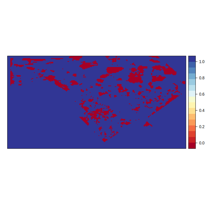
We can check the resulting grid by plotting the map.

spatialPlot(pvalGrid)

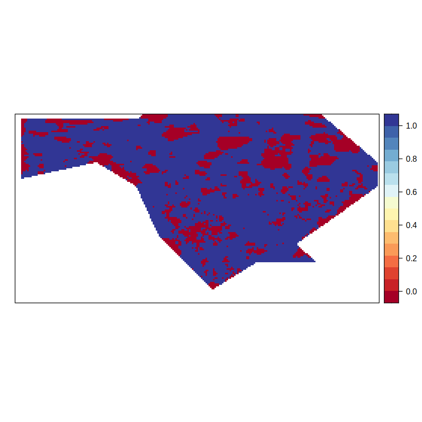
../_images/555c31759e46a341238dbc16ed2c1bc93af4d54ed78713c8e61bdcda5d84d69d.png

We build (binaryGrid) and apply (gridArithmetics) a mask to avoid R misusing NaN data out of the regions of interest when calculating the p-values.

mask <- binaryGrid(climatology(grid),condition = "GE", threshold = 0, values = c(NA,1))
pvalGrid <- gridArithmetics(pvalGrid, mask)

spatialPlot(pvalGrid)

../_images/3e4173119b7c1bb0abfe1f204da2b320916ca840d1f328890f4c25d73e063eef.png

We can now use the p-values computed above to add a hatching pattern over the trend maps. To do so, we encapsulate the function map.hatching in a 2-way loop that corresponds to each line in a ‘x’ symbol. An ‘x’ would be associated whenever the condition is fullfilled, in our case whenever at least half the gridpoints of the upscaled grid are non-significant (i.e., 0-valued in the binary p-value object, pvalGrid). We use the mean fuction as the upscaling aggregation function, moving from a spatial resolution of half a degree in the trends field, to 2 degrees in the hatching. The upscaled (hatching) grid resolution is based on the density parameter of function map.hatching. In our case density = 4 and, therefore, the corresponding spatial resolution is 4 x 0.5 degrees = 2 degrees.

hatching.lines <- lapply(c("45","-45"), FUN = function(angle) {
  c(map.hatching(clim = climatology(pvalGrid), 
                 threshold = 0.5, 
                 condition = "GE", 
                 density = 4,
                 angle = angle, coverage.percent = 50,
                 upscaling.aggr.fun = list(FUN = "mean", na.rm = TRUE)
  ), 
  "which" = 1, lwd = 0.5)
})

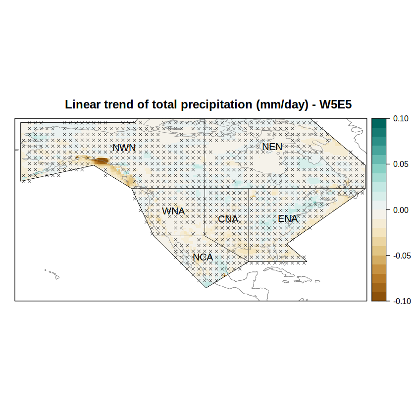
We rely again on spatialPlot from visualizeR to plot the trend maps and include the p-value as hatching as a member of the sp.layout argument list.

spatialPlot(trendGrid, 
            col.regions = brewer.pal(n = 9, "BrBG") %>% colorRampPalette(),
            at = seq(-0.1, 0.1, 0.01), 
            set.min = -0.1,
            set.max = 0.1,
            main = paste("Linear trend of total precipitation (mm/day) - W5E5"),
            sp.layout = list(
              hatching.lines[[1]],
              hatching.lines[[2]],  
              list(regs, first = FALSE, lwd = 0.6),
              list(coast, col = "gray50", first = FALSE, lwd = 0.6),  
              list("sp.text", coordinates(regs), names(regs), first = FALSE, cex = 1)
            )
)

../_images/f6e6af5a554cdc20e37d77d56edaad955a3191f3af34337f12107ae28c31f667.png

Anomaly time series#

Finally, we can have a look at the trends in average time series for each IPCC region. For this purpose, we loop over the IPCC regions to crop the field for each particular region. This will facilitate the spatial averaging over each region. To do so we rely on function overGrid.

grid.regs <- lapply(names(regs), function(r) overGrid(grid, regs[r]))

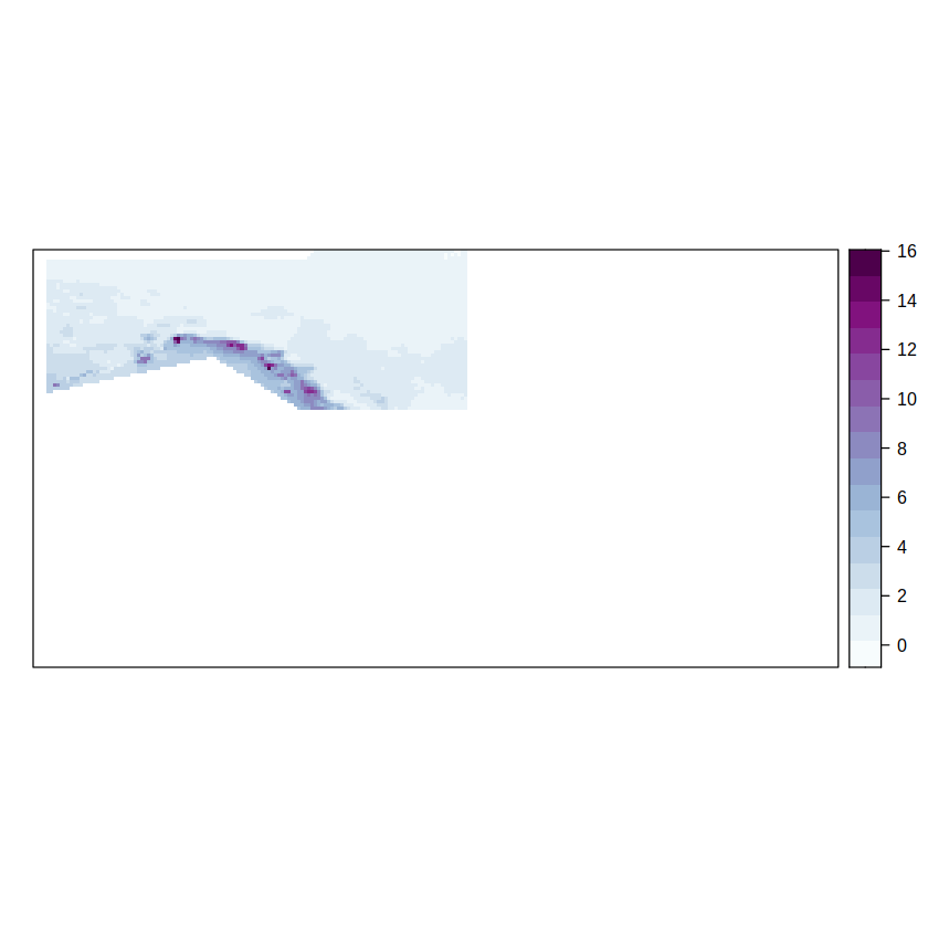
Let’s check the corresponding map e.g. for NWN

spatialPlot(climatology(grid.regs[["NWN"]]), 
            col.regions = brewer.pal(n = 9, "BuPu") %>% colorRampPalette()
)

[2023-05-07 16:59:41] - Computing climatology...

[2023-05-07 16:59:41] - Done.

../_images/95d007172d6769e1d6587ca50c15917809859f6d213d5210df1eff088219e8c6.png

We compute the anomalies by calling scaleGrid of transformeR and setting the argument type = center to substract the mean from the temporal series. Previously, we call aggregateGrid over the list of IPCC objets to average spatially over each region and, therefore, output the temporal series for every North American IPCC region.

spatial.mean <- function(grid) aggregateGrid(grid, aggr.spatial = list(FUN = "mean", na.rm = TRUE)) %>% scaleGrid(type = "center")
grid.anom <- lapply(grid.regs, spatial.mean)  

[2023-05-07 16:59:42] - Scaling ...

Calculating areal weights...

[2023-05-07 16:59:42] - Aggregating spatially...

[2023-05-07 16:59:42] - Done.

[2023-05-07 16:59:42] - Done

[2023-05-07 16:59:42] - Scaling ...

Calculating areal weights...

[2023-05-07 16:59:42] - Aggregating spatially...

[2023-05-07 16:59:42] - Done.

[2023-05-07 16:59:42] - Done

[2023-05-07 16:59:42] - Scaling ...

Calculating areal weights...

[2023-05-07 16:59:42] - Aggregating spatially...

[2023-05-07 16:59:42] - Done.

[2023-05-07 16:59:42] - Done

[2023-05-07 16:59:42] - Scaling ...

Calculating areal weights...

[2023-05-07 16:59:42] - Aggregating spatially...

[2023-05-07 16:59:42] - Done.

[2023-05-07 16:59:42] - Done

[2023-05-07 16:59:42] - Scaling ...

Calculating areal weights...

[2023-05-07 16:59:42] - Aggregating spatially...

[2023-05-07 16:59:42] - Done.

[2023-05-07 16:59:42] - Done

[2023-05-07 16:59:42] - Scaling ...

Calculating areal weights...

[2023-05-07 16:59:42] - Aggregating spatially...

[2023-05-07 16:59:42] - Done.

[2023-05-07 16:59:42] - Done

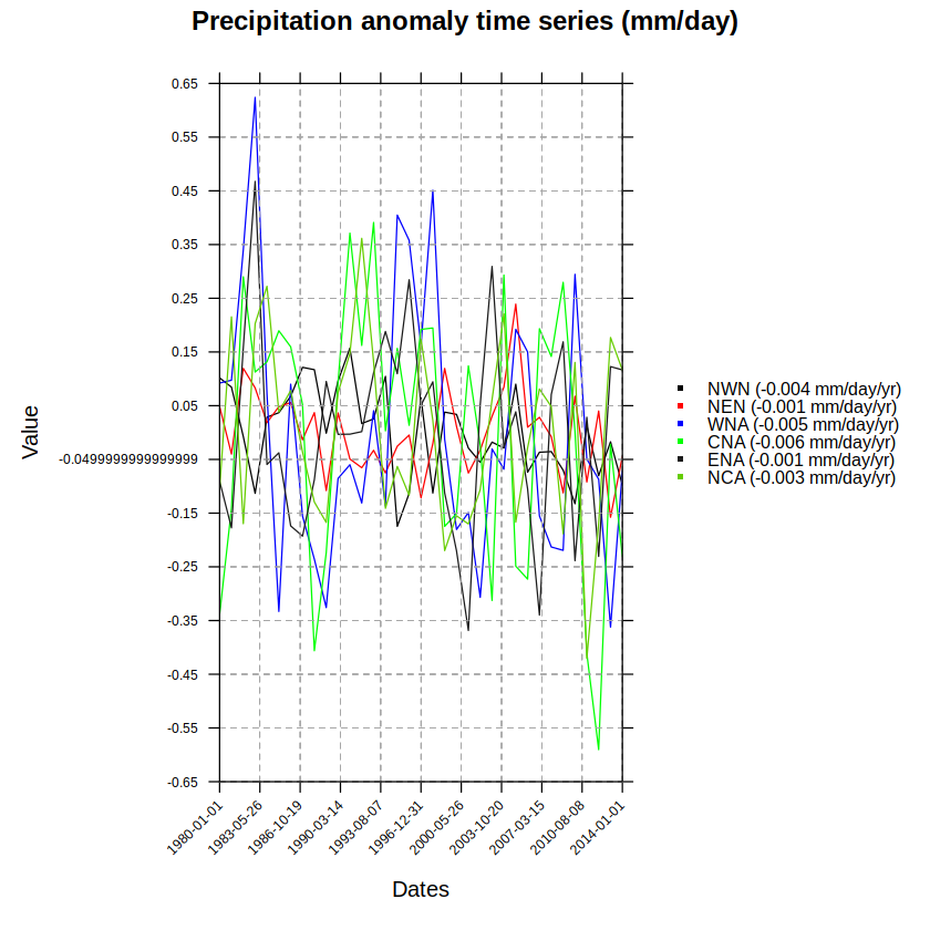
Finally, we will use temporalPlot (library visualizeR) to show these anomaly time series. temporalPlot uses the names of the grid objects to create the legend, region names in this case:

names(grid.anom)

'NWN'
'NEN'
'WNA'
'CNA'
'ENA'
'NCA'

If we’d like to add the trend value to the legend, we only need to paste these values to the names of object grid.anom before calling temporalPlot.

trend.val <- lapply(1:length(grid.anom), FUN = function(x) {
    aux <- linearTrend(grid.anom[[x]]) %>% subsetGrid(var = "b")
    round(aux$Data[1], digits = 3)
})
names(grid.anom) <- sprintf("%s (%g mm/day/yr)", names(grid.anom), trend.val)

The slope of the linear trend is estimated based on the temporal resolution of the data. Please consider using the function aggregateGrid prior to the call of linearTrend to adequate the data to your resolution of interest.

[2023-05-07 16:59:42] - Computing climatology...

[2023-05-07 16:59:42] - Done.

Warning message:
“Only one grid passed as input. Nothing was done”

The slope of the linear trend is estimated based on the temporal resolution of the data. Please consider using the function aggregateGrid prior to the call of linearTrend to adequate the data to your resolution of interest.

[2023-05-07 16:59:42] - Computing climatology...

[2023-05-07 16:59:42] - Done.

Warning message:
“Only one grid passed as input. Nothing was done”

The slope of the linear trend is estimated based on the temporal resolution of the data. Please consider using the function aggregateGrid prior to the call of linearTrend to adequate the data to your resolution of interest.

[2023-05-07 16:59:42] - Computing climatology...

[2023-05-07 16:59:42] - Done.

Warning message:
“Only one grid passed as input. Nothing was done”

The slope of the linear trend is estimated based on the temporal resolution of the data. Please consider using the function aggregateGrid prior to the call of linearTrend to adequate the data to your resolution of interest.

[2023-05-07 16:59:42] - Computing climatology...

[2023-05-07 16:59:42] - Done.

Warning message:
“Only one grid passed as input. Nothing was done”

The slope of the linear trend is estimated based on the temporal resolution of the data. Please consider using the function aggregateGrid prior to the call of linearTrend to adequate the data to your resolution of interest.

[2023-05-07 16:59:42] - Computing climatology...

[2023-05-07 16:59:42] - Done.

Warning message:
“Only one grid passed as input. Nothing was done”

The slope of the linear trend is estimated based on the temporal resolution of the data. Please consider using the function aggregateGrid prior to the call of linearTrend to adequate the data to your resolution of interest.

[2023-05-07 16:59:42] - Computing climatology...

[2023-05-07 16:59:42] - Done.

Warning message:
“Only one grid passed as input. Nothing was done”

names(grid.anom)

'NWN (-0.004 mm/day/yr)'
'NEN (-0.001 mm/day/yr)'
'WNA (-0.005 mm/day/yr)'
'CNA (-0.006 mm/day/yr)'
'ENA (-0.001 mm/day/yr)'
'NCA (-0.003 mm/day/yr)'

temporalPlot(grid.anom,
               xyplot.custom = list(
                 main = "Precipitation anomaly time series (mm/day)", ylim=c(-0.65, 0.65)
               ))      

pad applied on the interval: year

pad applied on the interval: year

pad applied on the interval: year

pad applied on the interval: year

pad applied on the interval: year

pad applied on the interval: year

../_images/37ce15ee26665175cfdcf1d18c2155f2fd1762eaaef85d79e98dcdac019f896f.png

Session info#

sessionInfo()

Show code cell output Hide code cell output

R version 3.6.3 (2020-02-29)
Platform: x86_64-conda-linux-gnu (64-bit)
Running under: Fedora Linux 38 (Workstation Edition)

Matrix products: default
BLAS/LAPACK: /home/phanaur/mambaforge/envs/tfg/lib/libopenblasp-r0.3.21.so

locale:
 [1] LC_CTYPE=es_ES.UTF-8          LC_NUMERIC=C                 
 [3] LC_TIME=es_ES.UTF-8           LC_COLLATE=es_ES.UTF-8       
 [5] LC_MONETARY=es_ES.UTF-8       LC_MESSAGES=es_ES.UTF-8      
 [7] LC_PAPER=es_ES.UTF-8          LC_NAME=es_ES.UTF-8          
 [9] LC_ADDRESS=es_ES.UTF-8        LC_TELEPHONE=es_ES.UTF-8     
[11] LC_MEASUREMENT=es_ES.UTF-8    LC_IDENTIFICATION=es_ES.UTF-8

attached base packages:
[1] stats     graphics  grDevices utils     datasets  methods   base     

other attached packages:
 [1] rgdal_1.5-16            RColorBrewer_1.1-2      sp_1.4-5               
 [4] magrittr_2.0.1          climate4R.indices_0.2.0 geoprocessoR_0.2.0     
 [7] visualizeR_1.6.1        transformeR_2.1.3       loadeR_1.7.1           
[10] climate4R.UDG_0.2.3     loadeR.java_1.1.1       rJava_1.0-4            

loaded via a namespace (and not attached):
 [1] viridis_0.6.1           maps_3.3.0              foreach_1.5.1          
 [4] jsonlite_1.7.2          viridisLite_0.4.0       R.utils_2.10.1         
 [7] SpecsVerification_0.5-3 dotCall64_1.0-1         kohonen_3.0.10         
[10] sm_2.2-5.6              latticeExtra_0.6-29     pillar_1.6.1           
[13] lattice_0.20-44         glue_1.4.2              RcppEigen_0.3.3.9.1    
[16] uuid_0.1-4              digest_0.6.27           colorspace_2.0-1       
[19] R.oo_1.24.0             htmltools_0.5.1.1       Matrix_1.3-3           
[22] pkgconfig_2.0.3         raster_3.4-10           padr_0.5.3             
[25] purrr_0.3.4             scales_1.1.1            jpeg_0.1-8.1           
[28] CircStats_0.2-6         dtw_1.22-3              tibble_3.1.2           
[31] proxy_0.4-25            generics_0.1.0          ggplot2_3.3.3          
[34] ellipsis_0.3.2          repr_1.1.3              verification_1.42      
[37] pbapply_1.4-3           gdalUtils_2.0.3.2       convertR_0.2.0         
[40] crayon_1.4.1            easyVerification_0.4.4  evaluate_0.14          
[43] R.methodsS3_1.8.1       fansi_0.4.2             MASS_7.3-54            
[46] tools_3.6.3             data.table_1.14.0       lifecycle_1.0.0        
[49] munsell_0.5.0           akima_0.6-2.1           compiler_3.6.3         
[52] mapplots_1.5.1          rlang_0.4.11            grid_3.6.3             
[55] RCurl_1.98-1.3          iterators_1.0.13        pbdZMQ_0.3-5           
[58] IRkernel_1.2            spam_2.6-0              bitops_1.0-7           
[61] tcltk_3.6.3             base64enc_0.1-3         boot_1.3-28            
[64] vioplot_0.3.6           codetools_0.2-18        gtable_0.3.0           
[67] abind_1.4-5             R6_2.5.0                gridExtra_2.3          
[70] zoo_1.8-9               dplyr_1.0.6             udunits2_0.13          
[73] utf8_1.2.1              parallel_3.6.3          IRdisplay_1.0          
[76] Rcpp_1.0.6              fields_12.3             vctrs_0.3.8            
[79] png_0.1-7               tidyselect_1.1.1       

References#

Atl: Atlas/reference-regions at main · IPCC-WG1/Atlas. https://github.com/IPCC-WG1/Atlas/tree/main/reference-regions.
Ini: Inicio | Servicio Climático de Datos. https://www.scds.es/es/.
WFD: WFDE5 over land merged with ERA5 over the ocean (W5E5). https://dataservices.gfz-potsdam.de/pik/showshort.php?id=escidoc:4855898.
Wha22: What is loadeR? Santander Meteorology Group (UC-CSIC), July 2022.
Cli22: climate4R.UDG. Santander Meteorology Group (UC-CSIC), June 2022.