Using the 4th version of the IPCC WGI reference regions in R

# Atlas notebooks

***

> This notebook reproduces and extends parts of the figures and products of the AR6-WGI Atlas. It is part of a notebook collection available at https://github.com/IPCC-WG1/Atlas for reproducibility and reusability purposes. This work is licensed under a [Creative Commons Attribution 4.0 International License](http://creativecommons.org/licenses/by/4.0).
>
> ![Creative Commons License >](https://i.creativecommons.org/l/by/4.0/88x31.png)

Using the 4th version of the IPCC WGI reference regions in R#

30/6/2021

M. Iturbide (Santander Meteorology Group. Institute of Physics of Cantabria. CSIC-University of Cantabria, Santander, Spain)

IPCC-WGI-reference-regions-v4 is the new set of reference regions that update the IPCC AR5 reference regions [AR5, n.d.] for reporting sub-continental climate information (e.g. CMIP6 projections). This tutorial shows how the standard R packages for spatial data can be used to manipulate and plot these regions, and how these capabilities can be further extended for climate data processing using the climate4R framework [The R-based climate4R Open Framework for Reproducible Climate Data Access and Post-Processing - ScienceDirect, n.d.].

Requirements:#

The following R packages are used to work with spatial data:

library(rgdal)
library(sp)
library(RColorBrewer)

and the climate4R components used to load, analyse and visualize climate data:

loadeR [An R Package to Visualize and Communicate Uncertainty in Seasonal Climate Prediction - ScienceDirect]: SantanderMetGroup/loadeR
visualizeR: SantanderMetGroup/visualizeR
transformeR: SantanderMetGroup/transformeR
geoprocessoR: SantanderMetGroup/geoprocessoR

See installation details and options, including a conda recipe, in the climate4R main repository.

Using the updated IPCC regions:#

Import the reference regions:#

From shapefile: the shapefile of IPCC-WGI-reference-regions-v4 is available for download at the Atlas GitHub repository [Repository Supporting the Implementation of FAIR Principles in the IPCC-WGI Atlas, 2022], within the reference-regions subdirectory stored in a .zip file (shapefiles consist of a number of complementary files storing geo-reference information, geometries, the associated database etc.). In this example, we first extract the zip contents into a temporary directory for data import.

Function readOGR from package rgdal loads shapefiles into the R environment.

tmpdir <- tempdir()
unzip("../reference-regions/IPCC-WGI-reference-regions-v4_shapefile.zip", exdir = tmpdir)
refregions <- readOGR(dsn = tmpdir, layer = "IPCC-WGI-reference-regions-v4")

The R object that is obtained is a SpatialPolygonsDataFrame, this is a Spatial* class object from package sp.

class(refregions)

'SpatialPolygonsDataFrame'

From R object: the refregions R object is also available in the same repo directory, thus, the Spatial object of the regions can be directly loaded into R as follows:

load("../reference-regions/IPCC-WGI-reference-regions-v4_R.rda", verbose = TRUE)

We can simplify this object by converting it to a SpatialPolygons class object (i.e., only the polygons are retained and their attributes discarded):

refregions <- as(IPCC_WGI_reference_regions_v4, "SpatialPolygons")

Plotting regions:#

We can use function plot to visualize the regions:

plot(refregions)

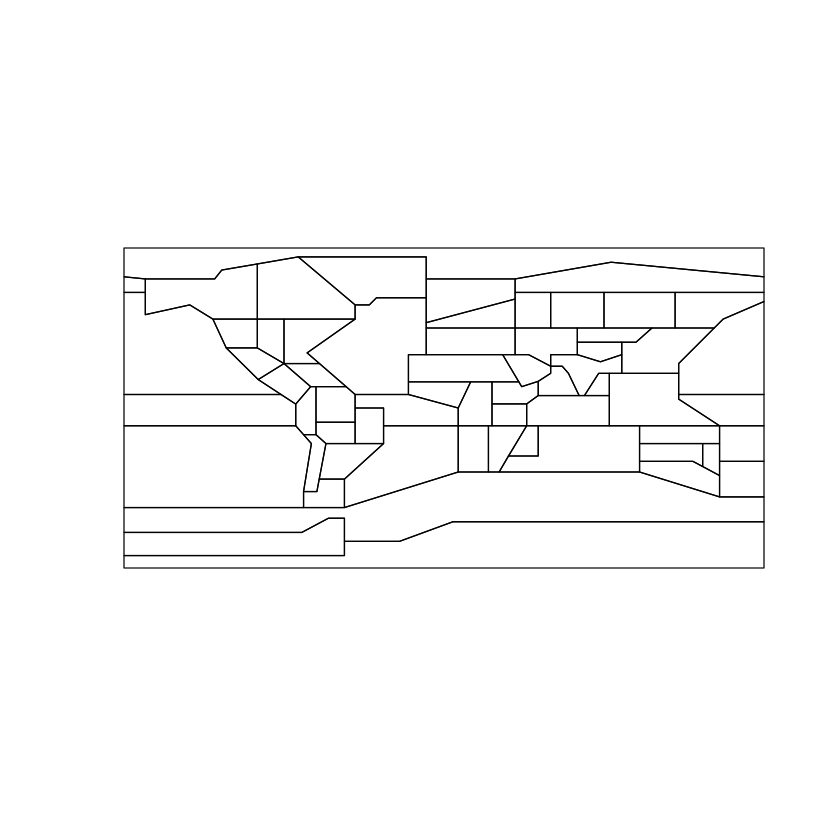
../_images/35a645e7e432e20f5519bc57e3173f2f1eddf7955a66851a563a880b0b9606bc.png

The R basic plotting functions allow adding layers to the plot. Here the region names and coastline are added. Shapefiles such as global coastlines and other physical features or administrative boundaries can be either read from local or obtained from the Internet. In this example, a world coastline layer is used from the Natural Earth [Natural Earth - Free Vector and Raster Map Data at 1:10m, 1:50m, and 1:110m Scales, n.d.] public repository of digital cartography.

(begin example)

An example follows on how to download and load the vector layer. However, note that this step can be skipped and read the layer directly from the auxiliary-material subdir.

The target vector layer (shapefile format) is next downloaded from Natural Earth download site to a temporary file and extracted:

temp.dir <- tempdir()
zipfile <- file.path(temp.dir, "world.zip")
download.file(url = "https://www.naturalearthdata.com/http//www.naturalearthdata.com/download/110m/physical/ne_110m_coastline.zip",
              destfile = zipfile)
unzip(zipfile, exdir = temp.dir)

and next imported into R:

coastLines <- readOGR(dsn = temp.dir, layer = "ne_110m_coastline")

OGR data source with driver: ESRI Shapefile 
Source: "/tmp/RtmpTcyQ2r", layer: "ne_110m_coastline"
with 134 features
It has 3 fields
Integer64 fields read as strings:  scalerank 

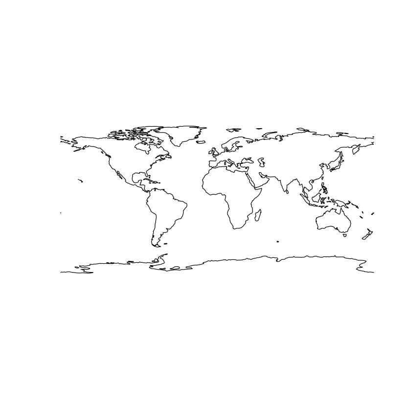
plot(coastLines)

../_images/cfa5dfcd8555161cb25e039a415bc697cd30c7423e3689d37d26ad513befbd21.png

(End of example)

However, for better reproducibility, the vector layer is already stored in the auxiliary-material subdirectory:

coastLines <- readOGR(dsn = "./auxiliary-material/", layer = "WORLD_coastline")

OGR data source with driver: ESRI Shapefile 
Source: "/home/phanaur/github/Atlas/notebooks/auxiliary-material", layer: "WORLD_coastline"
with 127 features
It has 2 fields

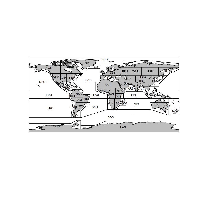
plot(coastLines, col = "grey")
plot(refregions, add = TRUE)
text(x = coordinates(refregions)[ ,1],
     y = coordinates(refregions)[ ,2],
     labels = names(refregions), cex = 0.6)

../_images/797b4d7767dd29bbd4455e772f8b6484843a31329b6aa5b7894a0459e595b2e3.png

Selecting specific regions#

The IDs of all regions can be inspected for easy subsetting:

names(names(refregions))

'GIC'
'NWN'
'NEN'
'WNA'
'CNA'
'ENA'
'NCA'
'SCA'
'CAR'
'NWS'
'NSA'
'NES'
'SAM'
'SWS'
'SES'
'SSA'
'NEU'
'WCE'
'EEU'
'MED'
'SAH'
'WAF'
'CAF'
'NEAF'
'SEAF'
'WSAF'
'ESAF'
'MDG'
'RAR'
'WSB'
'ESB'
'RFE'
'WCA'
'ECA'
'TIB'
'EAS'
'ARP'
'SAS'
'SEA'
'NAU'
'CAU'
'EAU'
'SAU'
'NZ'
'EAN'
'WAN'
'ARO'
'NPO'
'EPO'
'SPO'
'NAO'
'EAO'
'SAO'
'ARS'
'BOB'
'EIO'
'SIO'
'SOO'

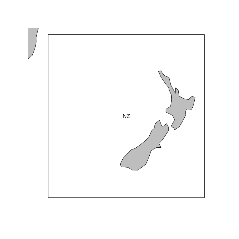
For instance, in order to extract one single region (e.g., New Zealand, NZ):

newzealand <- refregions["NZ"]
plot(newzealand)
plot(coastLines, col = "grey", add = TRUE)
text(x = coordinates(newzealand)[,1],
     y = coordinates(newzealand)[,2],
     labels = names(newzealand), cex = 1)

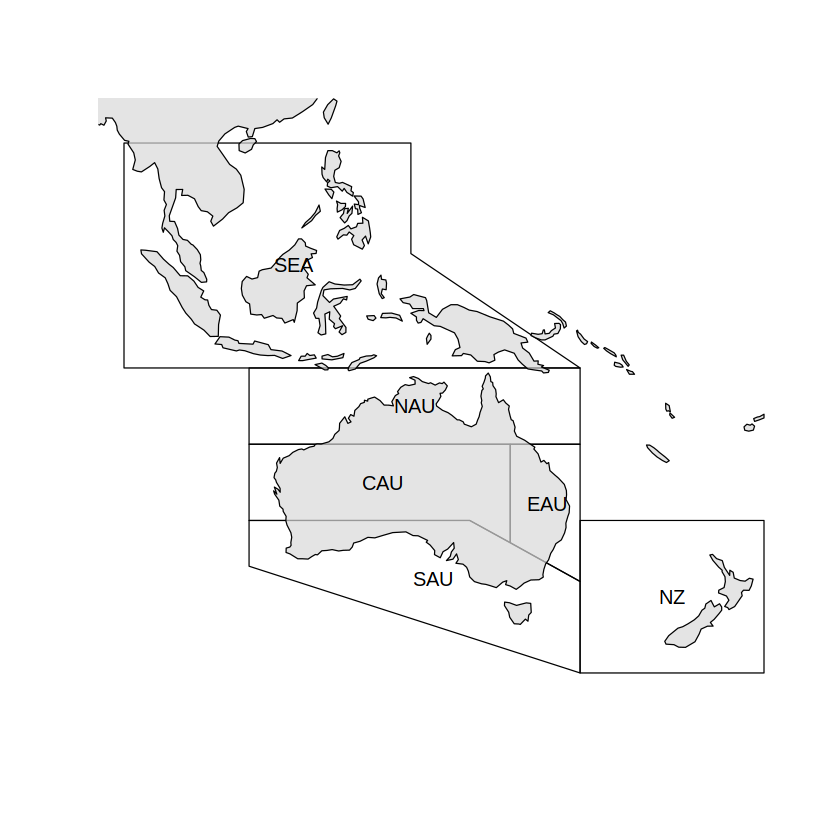
../_images/0af850764336d118dd2ad3f87bd8a90753c8d3ab1a0091514ca4ae8fd561b823.png

or several regions:

australasia <- refregions[c("NZ", "SEA", "NAU", "CAU", "EAU", "SAU")]

plot(australasia)
plot(coastLines, col = rgb(0.85,0.85,0.85,0.7), add = TRUE)
text(x = coordinates(australasia)[,1],
    y = coordinates(australasia)[,2],
    labels = names(australasia), cex = 1)

../_images/2cf5287cab215fa4cbbc1a7ba921058ca52c0b61bcddf62883a0bb03e0392321.png

Example:#

In this example we will consider a NetCDF file with historical temperature simulations and show several analysis and visualizations at a global scale or filtering by regions. To this aim, we load using climate4R an example dataset corresponding to the following ESGF request:

MIP Era: CMIP6
Source ID: CanESM5
Experiment ID: historical
Variant Label: r1i1p1f1
Table ID: Amon
Frequency: mon
Variable: tas

In this case, functions dataInventory and loadGridData (package loadeR) are used. First we need to install the climate4R framework (conda and docker installations available at SantanderMetGroup/ATLAS).

library(transformeR)
library(loadeR)
library(visualizeR)
library(geoprocessoR)

    _______   ____  ___________________  __  ________ 
   / ___/ /  / /  |/  / __  /_  __/ __/ / / / / __  / 
  / /  / /  / / /|_/ / /_/ / / / / __/ / /_/ / /_/_/  
 / /__/ /__/ / /  / / __  / / / / /__ /___  / / \ \ 
 \___/____/_/_/  /_/_/ /_/ /_/  \___/    /_/\/   \_\ 
 
      github.com/SantanderMetGroup/climate4R

transformeR version 2.1.3 (2021-08-04) is loaded

WARNING: Your current version of transformeR (v2.1.3) is not up-to-date

Get the latest stable version (2.1.4) using <devtools::install_github('SantanderMetGroup/transformeR')>

Please see 'citation("transformeR")' to cite this package.

Loading required package: rJava

Loading required package: loadeR.java

Java version 11x amd64 by Azul Systems, Inc. detected

NetCDF Java Library v4.6.0-SNAPSHOT (23 Apr 2015) loaded and ready

Loading required package: climate4R.UDG

climate4R.UDG version 0.2.3 (2021-07-05) is loaded

WARNING: Your current version of climate4R.UDG (v0.2.3) is not up-to-date

Get the latest stable version (0.2.4) using <devtools::install_github('SantanderMetGroup/climate4R.UDG')>

Please use 'citation("climate4R.UDG")' to cite this package.

loadeR version 1.7.1 (2021-07-05) is loaded

Please use 'citation("loadeR")' to cite this package.

visualizeR version 1.6.1 (2021-03-11) is loaded

Please see 'citation("visualizeR")' to cite this package.

geoprocessoR version 0.2.0 (2020-01-06) is loaded

Please see 'citation("geoprocessoR")' to cite this package.

First, dataInventory provides basic information about the variables available in the file/dataset:

di <- dataInventory("./auxiliary-material/CMIP6Amon_tas_CanESM5_r1i1p1f1_historical_gn_185001-201412.nc")
str(di)

As we can see from the inventory output, it contains a single variable (‘tas’, 2 meters air temperature). To load this data, the function loadGridData from package loadeR is used:

grid1 <- loadGridData(dataset = "./auxiliary-material/CMIP6Amon_tas_CanESM5_r1i1p1f1_historical_gn_185001-201412.nc",
                      var = "tas")

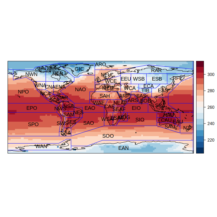
The example data is the temperature field for the period 1850-2014. In order to plot the first time step, we extract the data for January 1850 with the function subsetGrid (package transformeR):

grid185001 <- subsetGrid(grid1, years = 1850, season = 1, drop = TRUE)

spatialPlot from package visualizeR is the main map plotting function in climate4R. It is a wrapper of the powerful spplot method from package sp, thus accepting all possible optional parameters from lattice graphics. In addition, it also incorporates some additional arguments for straightforward fulfillment of commonplace requirements in climate data visualization (e.g. backdrop.theme, set.min, set.max, lonCenter, color.theme, rev.colors etc.).

regnameslayer <- list("sp.text", coordinates(refregions), names(refregions))
spatialPlot(grid185001, backdrop.theme = "coastline", 
            color.theme = "RdBu",
            rev.colors = TRUE,
            sp.layout = list(list(refregions, first = FALSE, col = "blue"), regnameslayer))

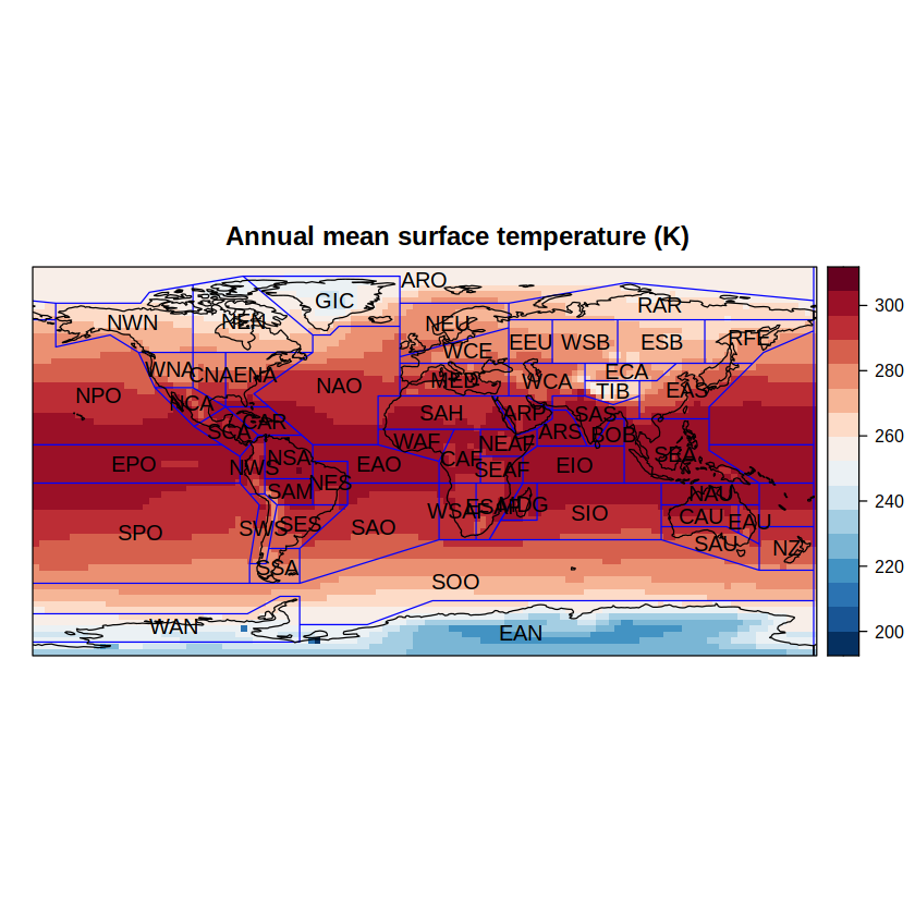
../_images/93f5bf38a9edcdc0effc8c1141757b6c57aa2c9e0ff5bb61544a152e69e23e24.png

We could also get the annual values using function aggregateGrid and plot the annual climatology:

grid1.ann <- aggregateGrid(grid1, aggr.y = list(FUN = "mean", na.rm = TRUE))
spatialPlot(climatology(grid1.ann), backdrop.theme = "coastline", 
            color.theme = "RdBu",
            rev.colors = TRUE,
            main = "Annual mean surface temperature (K)",
            sp.layout = list(list(refregions, first = FALSE, col = "blue"), regnameslayer))

[2023-05-07 17:01:32] Performing annual aggregation...

[2023-05-07 17:01:35] Done.

[2023-05-07 17:01:35] - Computing climatology...

[2023-05-07 17:01:35] - Done.

../_images/e2f825abf41ea8c021114fd4e9f9e0953604e7db3da93949de9367aa46648cc2.png

Extracting data for the region/s of interest#

Function overGrid perfoms the operation of intersecting a climate4R grid and a Spatial object. The only requirement is equal projections. Use function projectGrid to define and/or change the projection of a grid. Use proj4string and spTransform for Spatial objects. In this example the map projection is WGS84 (EPSG:4326). Note that several warning messages may appear during the following operations. These arise from recent changes in the versions of PROJ and GDAL, and can be safely ignored throughout these examples.

proj4string(refregions)

Warning message in proj4string(refregions):
“CRS object has comment, which is lost in output”

'+proj=longlat +ellps=WGS84 +no_defs'

An appropriate definition of the current coordinates projection will be later needed to ensure spatial consistency of geospatial operations:

grid1.ann <- setGridProj(grid = grid1.ann, proj = proj4string(refregions))

Warning message in proj4string(refregions):
“CRS object has comment, which is lost in output”

Once the spatial reference is defined, the spatial overlay is done:

grid1.au <- overGrid(grid1.ann, australasia)

Warning message in showSRID(uprojargs, format = "PROJ", multiline = "NO"):
“Discarded datum Unknown based on WGS84 ellipsoid in CRS definition”

spatialPlot(climatology(grid1.au), 
            color.theme = "RdBu",
            rev.colors = TRUE,
            sp.layout = list(coastLines, first = FALSE, col = "black"))

[2023-05-07 17:01:36] - Computing climatology...

[2023-05-07 17:01:36] - Done.

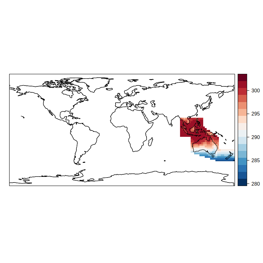
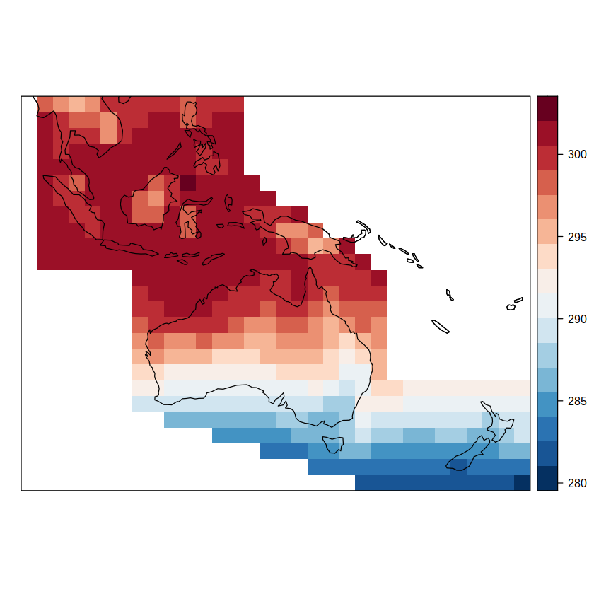
../_images/c09c76d8ebd862cb6f19044a15e295986832ec219c6884ce7baf08f7e8e76cff.png

Setting the argument subset = TRUE the spatial object is cropped to the region extent:

grid1.au <- overGrid(grid1.ann, australasia, subset = TRUE)

Warning message in showSRID(uprojargs, format = "PROJ", multiline = "NO"):
“Discarded datum Unknown based on WGS84 ellipsoid in CRS definition”

spatialPlot(climatology(grid1.au), 
            color.theme = "RdBu",
            rev.colors = TRUE,
            sp.layout = list(coastLines, first = FALSE, col = "black"))

[2023-05-07 17:01:36] - Computing climatology...

[2023-05-07 17:01:36] - Done.

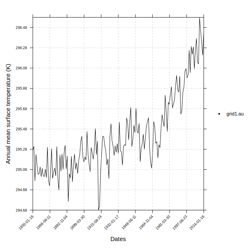
../_images/7bc2aad3705ea3f3b01c0a1e87a9826709c237b8073ce4b4736d6b2ee54b0c0b.png

Let’s calculate the regional average and visualize the yearly time series with temporalPlot:

temporalPlot(grid1.au, aggr.spatial = list(FUN = "mean", na.rm = TRUE), xyplot.custom = list(ylab = "Annual mean surface temperature (K)"))

pad applied on the interval: year

../_images/7d6de805b86c5d45c4f247cfcd785ca7560d291704531a5c21cbfa1cf57258e1.png

Session information#

sessionInfo()

Show code cell output Hide code cell output

R version 3.6.3 (2020-02-29)
Platform: x86_64-conda-linux-gnu (64-bit)
Running under: Fedora Linux 38 (Workstation Edition)

Matrix products: default
BLAS/LAPACK: /home/phanaur/mambaforge/envs/tfg/lib/libopenblasp-r0.3.21.so

locale:
 [1] LC_CTYPE=es_ES.UTF-8          LC_NUMERIC=C                 
 [3] LC_TIME=es_ES.UTF-8           LC_COLLATE=es_ES.UTF-8       
 [5] LC_MONETARY=es_ES.UTF-8       LC_MESSAGES=es_ES.UTF-8      
 [7] LC_PAPER=es_ES.UTF-8          LC_NAME=es_ES.UTF-8          
 [9] LC_ADDRESS=es_ES.UTF-8        LC_TELEPHONE=es_ES.UTF-8     
[11] LC_MEASUREMENT=es_ES.UTF-8    LC_IDENTIFICATION=es_ES.UTF-8

attached base packages:
[1] stats     graphics  grDevices utils     datasets  methods   base     

other attached packages:
 [1] geoprocessoR_0.2.0  visualizeR_1.6.1    loadeR_1.7.1       
 [4] climate4R.UDG_0.2.3 loadeR.java_1.1.1   rJava_1.0-4        
 [7] transformeR_2.1.3   RColorBrewer_1.1-2  rgdal_1.5-16       
[10] sp_1.4-5           

loaded via a namespace (and not attached):
 [1] viridis_0.6.1           maps_3.3.0              foreach_1.5.1          
 [4] jsonlite_1.7.2          viridisLite_0.4.0       R.utils_2.10.1         
 [7] SpecsVerification_0.5-3 dotCall64_1.0-1         kohonen_3.0.10         
[10] sm_2.2-5.6              latticeExtra_0.6-29     pillar_1.6.1           
[13] lattice_0.20-44         glue_1.4.2              RcppEigen_0.3.3.9.1    
[16] uuid_0.1-4              digest_0.6.27           colorspace_2.0-1       
[19] R.oo_1.24.0             htmltools_0.5.1.1       Matrix_1.3-3           
[22] pkgconfig_2.0.3         raster_3.4-10           padr_0.5.3             
[25] purrr_0.3.4             scales_1.1.1            jpeg_0.1-8.1           
[28] CircStats_0.2-6         dtw_1.22-3              tibble_3.1.2           
[31] proxy_0.4-25            generics_0.1.0          ggplot2_3.3.3          
[34] ellipsis_0.3.2          repr_1.1.3              pbapply_1.4-3          
[37] verification_1.42       gdalUtils_2.0.3.2       magrittr_2.0.1         
[40] crayon_1.4.1            easyVerification_0.4.4  evaluate_0.14          
[43] R.methodsS3_1.8.1       fansi_0.4.2             MASS_7.3-54            
[46] tools_3.6.3             data.table_1.14.0       lifecycle_1.0.0        
[49] munsell_0.5.0           akima_0.6-2.1           compiler_3.6.3         
[52] mapplots_1.5.1          rlang_0.4.11            grid_3.6.3             
[55] RCurl_1.98-1.3          iterators_1.0.13        pbdZMQ_0.3-5           
[58] IRkernel_1.2            spam_2.6-0              bitops_1.0-7           
[61] tcltk_3.6.3             base64enc_0.1-3         boot_1.3-28            
[64] vioplot_0.3.6           codetools_0.2-18        gtable_0.3.0           
[67] abind_1.4-5             R6_2.5.0                gridExtra_2.3          
[70] zoo_1.8-9               dplyr_1.0.6             utf8_1.2.1             
[73] parallel_3.6.3          IRdisplay_1.0           Rcpp_1.0.6             
[76] fields_12.3             vctrs_0.3.8             png_0.1-7              
[79] tidyselect_1.1.1       

References#

Sarkar D. (2008) Lattice: Multivariate Data Visualization with R. Springer, NY. ISBN 978-0-387-75968-5

Pac: An R package to visualize and communicate uncertainty in seasonal climate prediction - ScienceDirect. https://doi.org/10.1016/j.envsoft.2017.09.008.
App: Applied Spatial Data Analysis with R. https://asdar-book.org/.
Nat: Natural Earth - Free vector and raster map data at 1:10m, 1:50m, and 1:110m scales.
Rba: The R-based climate4R open framework for reproducible climate data access and post-processing - ScienceDirect. https://doi.org/10.1016/j.envsoft.2018.09.009.
CRA: CRAN - Package rgdal. https://cran.r-project.org/web/packages/rgdal/index.html.
atl22: Repository supporting the implementation of FAIR principles in the IPCC-WGI Atlas. IPCC-WG1, November 2022.
AR5: ipcc AR5. AR5 Regions. https://www.ipcc-data.org/guidelines/pages/ar5_regions.html.
Neu22: Erich Neuwirth. RColorBrewer: ColorBrewer Palettes. April 2022.